Download

1 / 33
330 likes | 436 Views
Identification of Regulatory Binding Sites Using Minimum Spanning Trees. Pacific Symposium on Biocomputing, pp. 327-338, 2003 Reporter: Chu-Ting Tseng Advisor: Prof. Chang-Biau Yang Date: Apr. 2, 2004. Outline. Introduction Minimum Spanning Tree (MST) Binding Site Identification by MST

E N D
Identification of Regulatory Binding Sites Using Minimum Spanning Trees Pacific Symposium on Biocomputing, pp. 327-338, 2003 Reporter: Chu-Ting Tseng Advisor: Prof. Chang-Biau Yang Date: Apr. 2, 2004
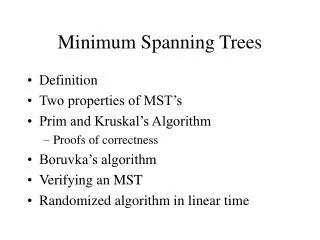
Outline • Introduction • Minimum Spanning Tree (MST) • Binding Site Identification by MST • Distance Scoring Function • Position-specific Information Content • Applications
Introduction • Computationally, the binding-site identification problem is often defined as to find short ”conserved” fragments, from a set of genomic sequences, which cover many (or all) of the provided genomic sequences.
Minimum spanning trees (MST) • It may be defined on Euclidean space points or on a graph. • G = (V, E): weighted connected undirected graph • Spanning tree: S = (V, T), T E, undirected tree • Minimum spanning tree(MST): a spanning tree with the smallest total weight.
An example of MST • A graph and one of its minimum costs spanning tree (sum=105)
Prim’s algorithm for finding MST Step 1: x V, Let A = {x}, B = V - {x}. Step 2: Select (u, v) E, u A, v B such that (u, v) has the smallest weight between A and B. Step 3: Put (u, v) in the tree. A = A {v}, B = B - {v} Step 4: If B = , stop; otherwise, go to Step 2. (see the example on the next page)
Binding Site Finding by MST (1) • Conceptually, we map all the fragments, collected from the provided genomic sequences, into a space so that similar fragments (on the sequence level) are mapped to nearby positions and dissimilar fragments to far away positions.
Binding Site Finding by MST (2) • Because of the relatively high frequency of the conserved binding sites appearing in the targeted genomic sequence regions, a group of such sites should form a “dense” cluster in a sparsely-distributed background. • If C is a cluster in D, then C’s data points form a subtree of the MST of D.
Binding Site Finding by MST (3) • If we plot the edge distance in the selection order by the Prim’s algorithm, with x-axis be the linear representation L(D) of D, and the y-axis represents the distance of the corresponding MST edge. Each cluster should form a “valley” in this plot. • A substring S of L(D) represents a cluster if and only if (a) S’s elements form a subtree, TS, of D’s MST, and (b) S’s both boundary edges have larger distances than any edge-distance of TS.
Binding Site Finding by MST (4) • For every substring of L(D) check whether it’s a cluster, it can be done linear time of the number of vertices. • Total time: O(||D||3)
Distance Scoring Function • For two k-mers A = a1…ak , B = b1…bk ∊ S, we define their distance ρ(A,B) = where M(x, y) = 0 if x = y otherwise 1. Initially, all σiis set to 1/K, where K is the number of sequences containing at least one of the k-mers A or B.
Method • Break the sequences into k-mers • Calculate the distance between each pair. • Apply the ClusterIdentification procedure to identify all clusters.
Conditions for a Cluster to Be a Binding Site • The position-specific information content of the gapless multiple-sequence alignment, among all the sequence fragments represented by a cluster, should be relatively high. • Elements of an identified cluster should not be among long, simple repeats • The data density within a cluster should be relatively higher than the one of the overall background.
Position-Specific Information Content where fb is the observed frequency of each base in the collection of sites and Pb is the fraction of each base in the genome.
Scoring Function using PSIC (1) • After a cluster is identified, we will measure the position specific information content. If the overall information content is lower than some threshold, we will discard this cluster for further consideration. • Otherwise…
Scoring Function using PSIC (2) • For each position i, we use its information content as σiin the next iteration. • Set M(ai, bi) = 2 - (pi(ai) + pi(bi)) + |pi(ai) -pi(bi)|, where pi(x) represents the frequency of letter x among all letters in position i.
Applications-- CRP (1) • CRP: Cyclic AMP receptor protein • CRP binding Sites: 18 sequences, each of length 105 bps, with 23 experimentally verified CRP binding sites (22-mers). • The only cluster identified consists of 24 fragments, of which 20 are known CRP sites.
Applications-- Yeast (1) • Yeast binding Sites: There are 8 regulatory sequences, each containing 1000 bp. • By using 9-mers, our method identified several clusters. The most populated cluster is TTACCACCG.
Applications-- Human (1) • Human binding Sites:113 regulatory sequences containing regulatory regions. Each sequence is 300 bp long, with 250 bp upstream and 50 bp downstream of the transcriptional start site.
Applications-- Human (2) • The GCAGCC motif with at most one mismatch appears in 96 regulatory sequences, even more frequently than the TATAAA motif, where appears in 66 regulatory sequences with at most one mismatch.
Reference • Stormo, G. D. and Hartzell III, G. W. “Identifying protein-binding sites from unaligned DNA fragments.” Proceedings of the National Academy of Sciences USA, Vol. 86, pp. 1183-1187, 1989.