Download
1 / 21
210 likes | 295 Views
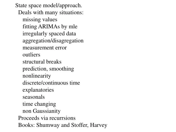
State space model/approach. Deals with many situations: missing values fitting ARIMAs by mle irregularly spaced data aggregation/ disagregation measurement error outliers structural breaks prediction, smoothing nonlinearity

E N D
State space model/approach. Deals with many situations: missing values fitting ARIMAs by mle irregularly spaced data aggregation/disagregation measurement error outliers structural breaks prediction, smoothing nonlinearity discrete/continuous time explanatories seasonals time changing non Gaussianity Proceeds via recurrsions Books: Shumway and Stoffer, Harvey
Details on Kalman Filter and Smoothing Code for Chapter 6 In astsa, there are three levels (0,1,2) of filtering and smoothing, Kfilter0/Ksmooth0, Kfilter1/Ksmooth1, Kfilter2/Ksmooth2. For various models, each script provides the Kalman filter/smoother, the innovations and the corresponding variance-covariance matrices, and the value of the innovations likelihood at the location of the parameter values passed to the script. MLE is then accomplished by calling the script that runs the filter. The model is specified by passing the model parameters. Level 0 is for the case of a fixed measurement matrix and no inputs; i.e., if At = A for all t, and there are no inputs, then use the code at level 0. If the measurement matrices are time varying or there are inputs, use the code at a higher level (1 or 2). Many of the examples in the text can be done at level 0. Level 1 allows for time varying measurement matrices and inputs, and level 2 adds the possibility of correlated noise processes. The models for each case are (x is state, y is observation, and t = 1, ..., n): ◊ Level 0: xt = Φ xt-1 + wt, yt = A xt + vt, wt ~ iidNp(0, Q) ⊥ vt ~ iidNq(0, R) ⊥ x0 ~ Np(μ0, Σ0)◊ Level 1: xt = Φ xt-1 + Υ ut + wt, yt = Atxt + Γ ut + vt, ut are r-dimensional inputs, etc.◊ Level 2: xt+1 = Φ xt + Υ ut+1 + Θ wt, yt = Atxt + Γ ut + vt, cov(ws, vt) = S δst, Θ is p × m, and wt is m-dimensional, etc. www.stat.pitt.edu/stoffer/tsa3
1 # Setup 2 y = cbind(gtemp,gtemp2); num = nrow(y); input = rep(1,num) 3 A = array(rep(1,2), dim=c(2,1,num)) 4 mu0 = -.26; Sigma0 = .01; Phi = 1 5 # Function to Calculate Likelihood 6 Linn=function(para){ 7 cQ = para[1] # sigma_w 8 cR1 = para[2] # 11 element of chol(R) 9 cR2 = para[3] # 22 element of chol(R) 10 cR12 = para[4] # 12 element of chol(R) 11 cR = matrix(c(cR1,0,cR12,cR2),2) # put the matrix together 12 drift = para[5] 13 kf = Kfilter1(num,y,A,mu0,Sigma0,Phi,drift,0,cQ,cR,input) 14 return(kf$like) } 15 # Estimation 16 init.par = c(.1,.1,.1,0,.05) # initial values of parameters 17 (est = optim(init.par, Linn, NULL, method="BFGS", hessian=TRUE, control=list(trace=1,REPORT=1))) 18 SE = sqrt(diag(solve(est$hessian)))
19 # display estimates 20 u = cbind(estimate=est$par, SE) 21 rownames(u)=c("sigw","cR11", "cR22", "cR12", "drift"); u estimate SE sigw 0.032730315 0.007473594 cR11 0.084752492 0.007815219 cR22 0.070864957 0.005732578 cR12 0.122458872 0.014867006 drift 0.005852047 0.002919058 22 # Smooth (first set parameters to their final estimates) 23 cQ=est$par[1] 24 cR1=est$par[2] 25 cR2=est$par[3] 26 cR12=est$par[4] 27 cR = matrix(c(cR1,0,cR12,cR2), 2) 28 (R = t(cR)%*%cR) # to view the estimated R matrix 29 drift = est$par[5] 30 ks = Ksmooth1(num,y,A,mu0,Sigma0,Phi,drift,0,cQ,cR,input) 31 # Plot 32 xsmooth = ts(as.vector(ks$xs), start=1880) 33 plot(xsmooth, lwd=2, ylim=c(-.5,.8), ylab="Temperature Deviations") 34 lines(gtemp, col="blue", lty=1) # color helps here 35 lines(gtemp2, col="red", lty=2)