Download
1 / 66
680 likes | 928 Views
Molecular phylogenetics. Xuhua Xia xxia@uottawa.ca http://dambe.bio.uottawa.ca. Biodiversity. “Tree-of-life”. Animals. Plants. Fungi. Endosymbiotic origin of chloroplasts (from cyanobacteria). Protists. Archaea. Bacterial origin of mitochondria. “Primitive” eukaryote. Bacteria.

E N D
Molecular phylogenetics Xuhua Xia xxia@uottawa.ca http://dambe.bio.uottawa.ca
Biodiversity Slide 2
“Tree-of-life” Animals Plants Fungi Endosymbiotic origin of chloroplasts (from cyanobacteria) Protists Archaea Bacterial origin of mitochondria “Primitive” eukaryote Bacteria Tips of branches represent extant organisms Cenancestor tolweb.org/tree/
Cenancestor The scientific consensus of the cenancestor is neither a single cell nor a single genome, but is instead an entangle bank of heterogeneous genomes with relatively free flow of genetic information. Out of this entangled bank of frolicking genomes arose probably many evolutionary lineages with horizontal gene transfer gradually reduced and confined within individual lineages. Only three (Archaea, Eubacteria, and Eukarya) of these early lineages have representatives survived to this day. Xia, X. and Q. Yang 2013. Cenancestor. In: S Maloy, K Hughes, editors. Brenner's Encyclopedia of Genetics, 2nd edition, Academic Press, San Diego. Volume1, pp. 493-494
Convergent Evolution Placental mammals Marsupials Slide 5
The Story of the German Farmer The elder son of the German Farmer: Strong and Robust Immunological & Electrophoretic Diagnosis German Farmer: Strong and Robust The younger son of the German Farmer: Weak and unmanly Slide 6
Three Kingdoms of Life Thermotoga Chloroflexus Escherichia Bacillus Rhodocyclus Mitochondria Rickettsia Dictyostelium Chloroplasts Zea Anacycsis Oxytricha Bacteria Saccharomyces Human Xenopus Thermococcus Trypanosoma Euglena Methanococcus Eucarya Methanobacterium Methanospirillum Sulfolobus Halococcus Thermoproteus Haloferax Archaea Slide 7
Where have all the whales gone? • Facts: • North Atlantic minke whales were not taken for commercial purposes under IWC resolutions since 1986 • Fin whales have not been hunted legally since 1986 • Hunting of humpback whales has been prohibited since 1966 • Birth rate was found to be higher than death rate • Why not more whales? • Illegal hunting? • Forensics Minke whele (North Atlantic) Sample #19a Sample #9 Sample #15 Sample #19b Humpback whale Sample #41 Sample #3 Sample #11 Sample WS4 Fin whale Slide 8
Where have all the turtles gone? Rookery Rookery Rookery Rookery Rookery Rookery Rookery Rookery Rookery Adult Feeding Grounds Slide 9
Conservation of the Green Turtle (a) Rookeries demographically independent Adult Feeding Grounds Rookery 1 Rookery 2 Rookery 3 (b) Rookeries demographically dependent Adult Feeding Grounds From Avise (1994, p 372) Slide 10
Mitochondrial DNA Variation Ind1 Rookery 1 Ind2 Ind3 Ind4 Ind5 Ind6 Rookery 2 Ind7 Ind8 Ind9 Ind10 Ind11 Rookery 3 Ind12 Ind13 Ind14 Ind15 Ind16 Rookery 4 Ind17 Ind18 (The original data set is far more extensive and complicated) Slide 11
these 4 are in same clade A B outgroup Time 1. Which tree is more accurate? trees are the same Mirror image of tree (or rotation of a clade) does not change the topology 2. Is the frog more closely related to the fish or to the human, based on this tree? node x representing common ancestor of frog & human is more recent than y (common ancestor of frog & fish) “The tree-thinking challenge” Science 310:979, 2005 NCBI PubMed website
PHYLOGENETIC TREES - display of evolutionary relationships among group of organisms - terminal Nodes - internal Branches - terminal - internal Branching pattern = topology OTUs = operational taxonomic units (eg species, individuals…) Fig. 5.1
Rooted vs unrooted trees Fig. 5.2 Root = common ancestor of all entities being studied Rooted tree has particular node which leads by a unique path to any other node # possible rooted vs. unrooted trees for 3 OTUs? for 4 OTUs…? (Fig. 5.5)
Scaled vs unscaled branches Branch length proportional to number of changes Fig. 5.3 Slide 15
True vs. inferred trees - only 1 true tree … … but usually must deal with inferred trees (based on certain data set and method of tree reconstruction) Score “similarities” - shared ancestral features - shared derived features - homoplasies (convergences, parallelism, reversals) ie. similarities of traits for reasons other than common ancestry
eg. living in different geographical locations Gene tree vs. species tree - genetic polymorphisms may be present in a population before it splits into 2 distinctly different populations - divergence time between 2 gene sequences may predate divergence time between 2 species Pop 1 Seq 1 Seq 2 Seq 3 Pop 2 Time “Gene splitting” time vs. speciation time
Gene tree vs species tree • Genetic polymorphisms may be present in a population before it splits into 2 distinctly different populations • - divergence time between 2 genes sequences may predate divergence time between 2 species - changes in DNA sequences can occur before or after speciation Gene tree may not always reflect species tree Fig. 5.6 Slide 18
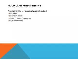
Phylogenetic tree reconstruction • Distance-based methods • Maximum parsimony methods • Maximum likelihood methods • Bayesian inference Slide 19
Distance-based methods • Objectives • Grasp the basic concepts distance-based tree-building algorithms • Learn the least-squares criterion and the minimum evolution criterion and how to use them to construct a tree • Distance-based methods • Genetic distance: generally defined as the number of substitutions per site. • JC69 distance • K80 distance • TN84 distance • F84 distance • TN93 distance • LogDet distance • Tree-building algorithms (UPGMA): • UPGMA • Neighbor-joining • Fitch-Margoliash • FastME Slide 20
Calculation of KJC69 AACGACGATCG: Species 1 AACGACGATCG AACGACGATCG: Species 2 t t The time is 2t between Species 1 to Species 2 Sp1: AAG CCT CGG GGC CCT TAT TTT TTG || | ||| ||| | ||| ||| || Sp2: AAT CTC CGG GGC CTC TAT TTT TTT p = 6/24 = 0.25 K = 0.304099 Genetic distances are scaled to be the number of substitutions per site. Slide 21
Numerical Illustration Sp1: AAG CCT CGG GGC CCT TAT TTT TTG || | ||| ||| | ||| ||| || Sp2: AAT CTC CGG GGC CTC TAT TTT TTT What are P and Q? P = 4/24, Q = 2/24 Comparison of distances: P = 0.25 Poisson P = -ln(1-p) = 0.288 KJC69 = 0.304099 KK80 = 0.3150786 Slide 22
A Star Tree (Completely Unresolved Tree) Human Chimpanzee Gorilla Orangutan Gibbon Slide 23
Genetic Distance Matrix Matrix of Genetic distances (Dij): Human Chimp Gorilla Orang GibbonHuman 0.015 0.045 0.143 0.198Chimp 0.030 0.126 0.179Gorilla 0.092 0.179Orang 0.179Gibbon 10 20 30 40 50 60 ----|----|----|----|----|----|----|----|----|----|----|----|-- human CAUGCUACUCCACACACCAAGCUAUCUAGCCUCCCCAAUCCAAAACAAACAUUAAACACUUU... chimpanzee CAUACUACUCCACACACCAAACUACCUAGCCUCCCCAAUCCAAAAUAAACAUCAAACACUUU... gorilla CAUACUACUCCACACACCAAAUCAUCUAGCCUCCCCAGUCCAGAACAAACACUGAAAAUUUU... orangutan CAUACCACUCCACACCCUAUACCAUCCAACUUCCCCUAUCCGAAACAAAUACAAAACACUUC... gibbon CAUACUACUCCAUACACCAAAUUAUCCAACUCCCCCAAUCCAGAAUAAACACCGACCAUCUU... *** * ****** ** * * * * * * **** *** ** *** * * * * Slide 24
UPGMA • Human Chimp Gorilla Orang GibbonHuman 0.015 0.045 0.143 0.198Chimp 0.030 0.126 0.179Gorilla 0.092 0.179Orang 0.179Gibbon • D(hu-ch),go = (Dhu,go + Dch,go)/2 = 0.038 D(hu-ch),or = (Dhu,or + Dch,or)/2 = 0.135D(hu-ch),gi = (Dhu,gi + Dch,gi)/2 = 0.189 • hu-ch Gorilla Orang Gibbonhu-ch 0.038 0.135 0.189Gorilla 0.092 0.179Orang 0.179Gibbon Human Chimp Gorilla Orang Gibbon Gorilla Orang Gibbon Human Chimp (hu,ch),(go,or,gi) Orang Gibbon Gorilla Human Chimp ((hu,ch),go),(or,gi) Slide 25
UPGMA • Human Chimp Gorilla Orang GibbonHuman 0.015 0.045 0.143 0.198Chimp 0.030 0.126 0.179Gorilla 0.092 0.179Orang 0.179Gibbon • D(hu-ch-go),or = (Dhu,or + Dch,or + Dgo,or)/3 = 0.120D(hu-ch-go),gi = (Dhu,gi + Dch,gi +Dgo,gi)/3 = 0.185 • hu-ch-go Orang Gibbonhu-ch-go 0.120 0.185Orangutan 0.179Gibbon • D(hu-ch-go-or),gi = (Dhu,gi + Dch,gi +Dgo,gi + Dor,gi)/4 = 0.184 Orang Gibbon Gorilla Human Chimp Gibbon Orang Gorilla Human Chimp (((hu,ch),go),or),gi) Slide 26
Phylogenetic Relationship from UPGMA • Human Chimp Gorilla Orang GibbonHuman 0.015 0.045 0.143 0.198Chimp 0.030 0.126 0.179Gorilla 0.092 0.179Orang 0.179Gibbon • hu-ch Gorilla Orang Gibbonhu-ch 0.038 0.135 0.189Gorilla 0.092 0.179Orang 0.179Gibbon • hu-ch-go Orang Gibbonhu-ch-go 0.120 0.185Orang 0.179Gibbon Slide 27
Branch Lengths ((hu,ch),(go,or,gi)) (((hu,ch),go),(or,gi)) ((((hu,ch),go),or),gi) Dhu-ch = 0.015 D(hu-ch),go = (Dhu,go + Dch,go)/2 = 0.038 D(hu-ch),or = (Dhu,or + Dch,or)/2 = 0.135D(hu-ch),gi = (Dhu,gi + Dch,gi)/2 = 0.189 D(hu-ch-go),or = (Dhu,or + Dch,or + Dgo,or)/3 = 0.120D(hu-ch-go),gi = (Dhu,gi + Dch,gi +Dgo,gi)/3 = 0.185 D(hu-ch-go-or),gi = (Dhu,gi + Dch,gi +Dgo,gi + Dor,gi)/4 = 0.184 0.0075 Human Chimp Gorilla Orang Gibbon 0.019 0.06 ((hu:0.0075,ch:0.0075),(go,or,gi)) (((hu:0.0075,ch:0.0075):0.019,go:0.019),(or,gi)) ((((hu:0.0075,ch:0.0075):0.0115,go:0.019):0.041,or:0.06):0.032,gi:0.092) 0.092 Slide 28
Final UPGMA Tree Human Chimp Gorilla Orang Gibbon 19 13 8 6 MY 0.092 0.060 0.019 0.0075 ((((hu:0.0075,ch:0.0075):0.0115,go:0.019):0.041,or:0.06):0.032,gi:0.092); Slide 29
Distance-based method • Distance matrix • Tree-building algorithms • UPGMA • Neighbor-joining • Fitch-Margoliash • FastME • Criterion-based methods: the least squares method • Branch-length estimation • Tree-selection criterion Slide 30
For three OTUs S1 x1 x3 S3 x2 S2 S1 S2 S3 S1 034S2 05S30 1 2 31 d12 d132 d233 d12 = x1 + x2 d13 = x1 + x3 d23 = x2 + x3 Slide 31
Least-square method 1 3 x3 x1 x5 x2 x4 2 4 4 Sp1 Sp2 0.3 Sp3 0.4 0.5 Sp4 0.4 0.6 0.6 d’12 = x1 + x2 d’13 = x1 + x5+ x3 d’14 = x1 + x5 + x4 d’23 = x2 + x5 + x3 d’24 = x2 + x5 + x4 d’34 = x3 + x4 4 Sp1 Sp2 d12 Sp3 d13 d23 Sp4 d14 d24 d34 Slide 32
The LS method in linear regression Y = a + b x RSS = 0 means a perfect fit of the linear model to the data. A large RSS means a poor fit. Slide 33
Least-square method 1 3 x3 x1 x5 Least-squares method: Find xi values that minimize SS x2 x4 2 4 d’12 = x1 + x2 d’13 = x1 + x5+ x3 d’14 = x1 + x5 + x4 d’23 = x2 + x5 + x3 d’24 = x2 + x5 + x4 d’34 = x3 + x4 (d12 - d’12)2= [d12 – (x1 + x2)]2 (d13 - d’13)2 = [d13 – (x1 + x5+ x3)]2 (d14 - d’14)2 = [d14 – (x1 + x5 + x4)]2 (d23 - d’23)2 = [d23 – (x2 + x5 + x3)]2 (d24 - d’24)2 = [d24 – (x2 + x5 + x4)]2 (d34 - d’34)2 = [d34 – (x3 + x4)]2 Slide 34
Least-squares method SS = [d12 – (x1 + x2)]2 + [d13 – (x1 + x5+ x3)]2 + [d14 – (x1 + x5 + x4)]2 + [d23 – (x2 + x5 + x3)]2+ [d24 – (x2 + x5 + x4)]2+ [d34 – (x3 + x4)]2 Take the partial derivative of SS with respective to xi, we have SS/x1 := -2 d12 + 6 x1 + 2 x2 - 2 d13 + 4 x5 + 2 x3 - 2 d14 + 2 x4 SS/x2 := -2 d12 + 2 x1 + 6 x2 - 2 d23 + 4 x5 + 2 x3 - 2 d24 + 2 x4 SS/x3 := -2 d13 + 2 x1 + 4 x5 + 6 x3 - 2 d23 + 2 x2 - 2 d34 + 2 x4 SS/x4 := -2 d14 + 2 x1 + 4 x5 + 6 x4 - 2 d24 + 2 x2 - 2 d34 + 2 x3 SS/x5 := -2 d13 + 4 x1 + 8 x5 + 4 x3 - 2 d14 + 4 x4 - 2 d23 + 4 x2 - 2 d24 Setting these partial derivatives to 0 and solve for xi, we have x1 = d13/4 + d12/2 - d23/4 + d14/4 - d24/4 x2 = d12/2 - d13/4 + d23/4 - d14/4 + d24/4, x3 = d13/4 + d23/4 + d34/2 - d14/4 - d24/4, x4 = d14/4 - d13/4 - d23/4 + d34/2 + d24/4, x5 = - d12/2 + d23/4 - d34/2 + d14/4 + d24/4 + d13/4 Slide 35
Least-squares method 1 3 x3 x1 x5 x2 x4 2 4 x1 = d13/4 + d12/2 - d23/4 + d14/4 - d24/4 x2 = d12/2 - d13/4 + d23/4 - d14/4 + d24/4, x3 = d13/4 + d23/4 + d34/2 - d14/4 - d24/4, x4 = d14/4 - d13/4 - d23/4 + d34/2 + d24/4, x5 = - d12/2 + d23/4 - d34/2 + d14/4 + d24/4 + d13/4 4 Sp1 Sp2 0.3 Sp3 0.4 0.5 Sp4 0.4 0.6 0.6 x1 = 0.075 x2 = 0.225 x3 = 0.275 x4 = 0.325 x5 = 0.025 Slide 36
Minimum Evolution Criterion 1 1 1 2 2 3 x3 x3 x3 x1 x1 x1 x5 x5 x5 x2 x2 x2 x4 x4 x4 4 2 3 4 4 3 The minimum evolution (ME) criterion: The tree with the shortest TreeLen is the best tree. Slide 37
Maximum Parsimony (MP) Method • Mapping character state changes to alternative topologies • Apply the maximum parsimony criterion to choose the best tree. • Efficient dynamic programming algorithm developed by Walter Fitch and David Sankoff • The only method with branch-and-bound search • Use only informative sites to discriminate among alternative topologies • Problems • Long-branch attraction • Failure to account to multiple substitutions Slide 38
Informative sites • A site with at least two different characters each being represented by at least two OTUs. • Meaningful only in Fitch Parsimony where all nucleotides or amino acids are equally likely to replace each other. • Sankoff parsimony introduces the step matrix and can use information in a "non-informative" site for discriminate among alternative topologies, e.g., when transitions and transversions are associated with different costs. Slide 39
Maximum parsimony method Informative sites: Fitch algorithm. Other sites can be informative with Sankoff algorithm 1 2 1 2 1 3 4 3 3 4 4 2 Dot = nt sub inferred on that branch Fig. 5.14 Slide 40
Maximum parsimony method Fig. 5.14 After analyzing all informative sites, add up all dots - tree with fewest is favoured tree Slide 41
Computing N1 • Each node is represented by a set of characters, with the terminal nodes (leaves) each represented by a set containing a single character. • The MP method traverses through each internal node, starting from the node closest to the leaves. • If two sets of the two daughter nodes have an empty intersection, then the node will be represented by the union of the two daughter sets, otherwise the node will be represented by the intersection. • Once the operation reaches the root, then the number of union operations is the minimum number of changes needed to map the site to the tree. Slide 42
Tree Length • Site 1 requires four union operations • Sites 3, 5, and 8 each require only one union operation • Sites 6 and 7, which are polymorphic with two nucleotide states but not informative, will require one change for any topology. • The tree length for the topology above: 4+(1+1+1)+(1+1) = 9 Slide 43
Criteria for a good estimator • Unbiased • Efficient • Consistent Slide 44
Inconsistency (Felsenstein, 1978) A B MP tree Model tree C A Rates or p p Branch lengths q p >> q Wrong q q B D C D • With more data the certainty that parsimony will give the wrong tree increases - so that parsimony is statistically inconsistent • It is now recognised that long-branch attraction is one of the most serious problems in phylogenetic inference Slide 45
Maximum likelihood Method • Likelihood L of a tree is the probability of observing the data given the treeL = P(data|tree) • Find the tree with the highest L value • Results depends on model of nucleotide substitution Slide 46
A example of Tree: Four sequences 2 1 3 4 A , C , G , T 3 2 1 1 5 6 5 6 5 6 4 4 Tree1 Tree2 Tree3 2 3 Unrooted tree for Sp1,Sp2,Sp3,Sp4 Number 5 and 6 stand for the two interior nodes whose nucleotides could be either A,C,G or T. Slide 47
Likelihood Method • The likelihood function for a nucleotide site(6-th site) is given by p6= Prob +Prob + … +Prob Site 1 2 3 4 5 6 7 8 9 10 Sp1 A C C A T G G T A A Sp2 A C A G T G C T A G Sp3 G C A G T C G T A G Sp4 G C A A C T C C A A Prob.: p1 p2 p3 p4 p5 p6 p7 p8 p9 p10 1(G) t1 t3 3(C) t5 5 6 t4 t2 4(T) 2(G) Tree1 16 Slide 48
Calculation of Likelihood 1(G) t1 t3 3(C) t5 5 6 t4 t2 4(T) 2(G) Tree1 where P(A),P(T),P(C),P(G) are empirical nucleotide frequencies satisfying P(A)+P(T)+P(C)+P(G)=1, Pii(t) and Pij(t) are given by JC69 • lnLTree1= ln(p1)+ln(p2)+…+ln(p10) • Calculate lnLTree2,lnLTree3 similarly. • We choose the tree which has the highest lnL i.e. Max(lnLTree1, lnLTree2 , lnLTree3 ). when Slide 49
Problems with ML method The ML method is strictly data-based. If we sampled 6 fish all being males, then our estimation of p is 6/6 = 1. Slide 50