Download
1 / 6
60 likes | 192 Views
Numerical Integration. Simpson’s Method. Trapezoid Method & Polygonal Lines

E N D
Numerical Integration Simpson’s Method
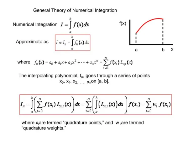
Trapezoid Method & Polygonal Lines One way to view the trapezoid method for integration is that the curves that you are attempting to estimate the integral of is being fitted with a polygonal line (a bunch of connected line segments) and then you compute the area under (or above) each line segment. f(x) b a Simpson’s Method Simpson’s method uses a second degree polynomial (i.e. a quadratic) to estimate the curve you are trying to find the integral of. This is a curve of the form y= c2x2+c1x+c0. The points are assumed to be evenly spaced. To get the estimate for the integral we will write out the 2nd degree polynomial using the data below to the right and then integrate it. c a c-h b c+h h h
We will begin with the special case with the value of c being zero. We begin by integrating the 2nd degree polynomial p(t)=c2t2+c1t+c0. We will simplify it some after integrating it. Substitute c0 and c2 values.
Shifting this over on any closed interval [a,b] we are interested in this becomes the same formula. On 2 partitions this formula becomes: f(x) b a In general this will become a kind of strange sum. Each of the function values will either be multiplied by 4 or 2 except for the first or the last. The number of subinterval points will need to be even.
Example Estimate the integral to the right with 4 subintervals. A partition with 3 subintervals can not be used here since 3 is odd. Partition size 2 In general the sum to estimate the integral can be split into 3 parts. One is the value at the two endpoints, the other two are the odd indexes and the even indexes. This is something important when it comes to implementation. even index odd index odd index even index
even index odd index odd index even index Algorithm for Simpson’s Method function intf( a, b, n) deltax = (b-a)/n isum = f(a)+f(b) oddsum=0 evensum=0 xodd=a+deltax xeven=xodd+deltax for(i=1,i(n/2)-1, i++, evensum = evensum + f(xeven) oddsum = oddsum + f(xodd) xodd = xodd + 2*deltax xeven = xodd + deltax) oddsum = oddsum + f(b-deltax) intf = (1/3)*deltax * (intsum+4*oddsum+2*evensum) prevint = intf(a, b, 2) nextint = intf(a, b, 4) for( i = 3, imaximum iterations && |prevint – nextint| error, i++, prevint = nextint nextint = intf(a , b, 2i)