Download
1 / 69
690 likes | 700 Views
Principle of Computed tomography. 嘉義長庚放射科 廖書柏. Introduction. In 1950 , Allan M. Cormack develop the theoretical and mathematical methods used to reconstruct CT images.

E N D
Principle of Computed tomography 嘉義長庚放射科 廖書柏
Introduction • In 1950,Allan M. Cormackdevelop the theoretical and mathematical methods used to reconstruct CT images. • In 1972Godfrey N. Hounsfield and colleagues of EMI Central Research Laboratories built the first CAT scan machine, taking Cormack's theoretical calculation into a real application. • For their independent efforts, Cormack and Hounsfield shared the Nobel Prize in medicine and physiology in 1979.
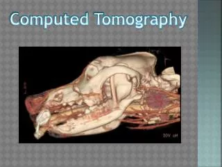
What is CT scanner? • A X-ray device capable of cross-section imaging -creates images of “slice” through patient
Advantages of CT scanning • Ability of differentiate overlying structure • Excellent contrast -overlying structure don’t decrease contrast -digital images, so variable window settings
X-ray Source and detectors • Source -rotating anode disk -small focus spot (down to 0.6 mm) -polychromatic beam • Detectors -xenon -solid-state: NaI(Tl)、CsI scintillaton crystals、 ceramic materials containing rare-earth oxides、BGO and CdWO4
xenon xenon Pressured xenon gas ionization Electrical signal
Solid-state Solid state Ceramic or crystal scintillatior Photon capture Light Photo-diode Electrical signal
Collimators • Pre-patient collimator- control slice thickness • Pre-detector collimator-reduce scattered radiation
Variations in scanner design based on : X-ray tube and detector movement Detector arrangement Rotating mechanism
First-generation ~1972 • single X-ray tube and one detector element • Pencil beam • about 5 minutes per slice from 180 degrees rotation. Translate-rotate movement
Second-generation ~1975 • Single X-ray tube and multiple detector elements • Narrow fan beam(~10。) • About one minute per slice Translate-rotate movement
Third-generation ~1975 • Single X-ray tube, rotating movement • Multiple detectors in curvilinear design, rotating movement • Fan beam(~30。) • Several seconds per slice Rotate-rotate movement
Fourth-generation ~1976 • Single X-ray tube, rotating movement • Fixed ring as many as 8000 detectors inside of gantry • 1-s scan time • Avoiding ring artifact problem of 3rd generation scanner Rotate-stationary movement
Fifth-generation ~1984 • four semicircular tungsten target rings spanning 210 degrees about the patient • Multiple detectors of two banks, fixed inside of the gantry • no mechanical movement • By using four target rings and two detector banks, eight slices of the patient may be imaged without moving patient.
EBCT( electron beam CT) A sub-second scanner, called “Imatron”
Each sweep of a target ring requires 50 ms and 8 ms delay to reset the beam. eight parallel slices (scanned two per sweep) requires approximately 224 milliseconds to complete
Sixth-generation ~1989 • Helical /spiral CT was introduced in 1989, based on Generation Three • Single X-ray tube and single-row detector • Never-stop and one-direction rotating X-ray tube, detectors • Capability to achieve one second image acquisition, or even sub-second • Slip ring replaced with the x-ray tube voltage cables enable continual tube rotation.
Slip ring technology in 1985 Slip ring allow continuous gantry rotation
Seventh-generation ~1998 • Single X-ray tube,Multiple-row detector, rotating movement • Allow simultaneous acquisition of multiple slice in a single rotation • Half-second rotation(0.5 s) • Sub-second scanner
The Basic CT Term • Image matrix • Linear attenuation coefficient • CT numbers
Image matrix • Every CT slice is subdivided into a matrix of up to 1024X1024 volume element (voxel) • The viewed image is then reconstructed as a corresponding matrix of picture element (pixel) • Each pixel is assigned a numerical value (CT number), which is the average of all the attenuation values contained within the corresponding voxel.
Voxel size= pixel size X slice thickness • The diameter of image reconstruction is called the field of view (FOV). Pixel size=FOV/matrix size
Linear Attenuation Coefficient (μ) • Basic property of matter • Depends on x-ray energy and atomic number (Z) of materials. • Attenuation coefficient reflects the degree to which x-ray intensity is reduced by a material x I0 I I = I0 e-μx
I0 I I = I0 e-(μ1x1+μ2x2) I0 I n I = I0 e-Σμixi i=1 μ(x, y) is the linear attenuation coefficient for the material in the slice
CT numbers • The precise CT number of any given pixel is calculated from the X-ray attenuation coefficient of the tissue contained in the voxel. • CT number ranged from -1000~3095(12 bit) k When k=1000, the CT numbers are Hounsfield units
CT numbers normalized in this manner provide a range of several CT numbers for 1% change in attenuation coefficient. Linear attenuation coefficient of various body tissues for 60 keV x-ray
Image reconstruction • The image is reconstructed from projections by a process called Filtered Backprojection. • "Filtered" refers to use digital algorithms called convolution to improve image quality or change certain image quality characteristics, such as detail and noise • "Backprojection" is the actual process used to produce or "reconstruct" the image.
The filtered backprojection process involves the following steps: • generating a sinogram from a set of N projections • filtering the data to compensate for blurring • Backprojecting the data .
Projection and sinogram • Ray: the X-ray read by every one detector within a short time interval. • Projection: all rays sum in a direction • Sinogram: all projections y P(t) t p x μ(x,y) t Sinogram X-rays
Filter • a de-blurring function is combined (convolved) with the projection data to remove most of the blurring before the data are backprojected. • A high-frequency filter reduces noise and makes the image appear “smoother.” • A low-frequency filter enhances edges and makes the image “shaper.” A low-frequency filter may be referred to as a “high-pass” filter because it suppresses low frequencies and allows high frequencies to pass.
Backprojection • Projection data (in Sinogram) 1D-FT filled in k-space central slice projection theorem 2D-inverse FT CT images 中央切面投影理論 (Central Slice Projection Theorem, CSPT): If a 1D Fourier Transform is performed on a projection of an object of some angle, the result will be identical to one line on 2D Fourier Transform of that object and at that angle.
Central Slice Projection Theorem ky y P(t) t F[P(t)] x kx μ(x,y) F(kx,ky) CSPT can relate the Fourier transform of the projection to one line in the 2D K space formed by the 2D Fourier transform of μ(x,y)
y v F-1[F(kx,ky)] x u u(x,y) F(kx,ky) ky kx Inverse 2D-FT
object 1D-FT image Inverse 2D-FT
Filtered backprojection Filtered backprojection removes the star-like blurring seen in simple backprojection.
Image manipulation • Image manipulation belongs to the domain of digital image processing.
Window width and level • The window width covers CT numbers of all the tissue of interest that is displayed as shades of gray, ranging from black to white. Thus width controls the contrast in the displayed image. • The level control adjust the center of the window and identifies the type of tissue to be imaged.
Reducing window width increases the displayed image contrast among the tissues
WL= 40 WW= 350 WL= -600 WW=1500
Pitch • Pitch is defined as the patient couch movement per rotation divided by the slice thickness. • Pitch= couch movement per rotation beam collimation Couch movement Slice thickness pitch 5 mm/rot 5 mm 5/5=1 10 mm/rot 5 mm 10/5=2