Download
1 / 42
420 likes | 608 Views
Discover the power of convolutional neural networks in deep learning, extracting abstract data representations through multiple non-linear transformations. Learn how different layers achieve varying levels of abstraction, from edges to familiar objects, with adaptable kernels and activation functions. Uncover the importance of detecting minute differences while ignoring irrelevant variations for successful machine learning. Explore the techniques like gradient descent, convolution, kernel operations, and parameter sharing. Dive into recent advancements and practical applications in CNN technology for enhanced data representation.

E N D
Neural networks (2) Convolutional neural network Goodfellow, Bengio,Courville, “Deep Learning” Gu et al. “Recent Advances in Convolutional Neural Networks” Le, “A tutorial on Deep Learning”
The purpose Data Features Model • Finding the correct features is critical in the success. • Kernels in SVM • Hidden layer nodes in neural network • Predictor combinations in RF • A successful machine learning technology needs to be able to extract useful features (data representations) on its own. • Deep learning methods: • Composition of multiple non-linear transformations of the data • Goal: more abstract – and ultimately more useful representations IEEE Trans Pattern Anal Mach Intell. 2013 Aug;35(8):1798-828
The purpose Learnrepresentations of data with multiple levels of abstraction Example: image processing Layer 1: presence/absence of edge at particular location & orientation. Layer 2: motifs formed by particular arrangements of edges; allows small variations in edge locations Layer 3: assemble motifs into larger combinations of familiar objects Layer 4 and beyond: higher order combinations Key: the layers are not designed by an engineer, but learned from data using a general-purpose learner. Nature. 521:436-444
The purpose • Key to success: • Detect minute differences • Ignore irrelevant variations Nature. 521:436-444
The purpose IEEE Trans Pattern Anal Mach Intell. 2013 Aug;35(8):1798-828 Nature 505, 146–148
The purpose Nature. 521:436-444
Reminder Common f(): rectified linear unit (ReLU) f(z) = max(0,z) c, The equations used for computing the forward pass in a neural net with two hidden layers and one output layer, each constituting a module through which one can backpropagate gradients. At each layer, we first compute the total input z to each unit, which is a weighted sum of the outputs of the units in the layer below. Then a non-linear function f(.) is applied to z to get the output of the unit. Nature. 521:436-444
Reminder d, The equations used for computing the backward pass. At each hidden layer we compute the error derivative with respect to the output of each unit, which is a weighted sum of the error derivatives with respect to the total inputs to the units in the layer above. We then convert the error derivative with respect to the output into the error derivative with respect to the input by multiplying it by the gradient of f(z). At the output layer, the error derivative with respect to the output of a unit is computed by differentiating the cost function. Nature. 521:436-444
Activation functions Sigmoid tend to have very small derivative when value is away from 0; For lower layers,multiplication of many partial derivatives will result in smaller gradients, compared to the higher layers– require larger learning rate for lower layers.
Gradient descent methods Batch gradient descent: update the model after all training samples have been evaluated. Stochastic gradient descent: update the model for one or a few samples in the training set. Mini-batch (commonly used) update the model on small batches of training data. Could help to jump out of local optimum Faster update when the gradient from a subset is stable.
CNN Convolution: 1D: A weighted average at each point Discrete case: 2D: Inmachine learning, often cross-correlation (without kernel flipping) is used but called convolution. Convolution surfaces in computer graphics, A Sherstyuk - 1998
CNN A kernel: The discrete convolution:
CNN Convolution achieves: Sparse connectivity – kernel smaller than the input Parameter sharing – One set of weights for one kernel Equivarianceto translation – Move the object in the input, its representation will move the same amount in the output
CNN A convolution layer is composed of several convolution kernels which are used to compute different feature maps For each feature map, the kernel is shared by all spatial locations of the input location (i,j) in the k-th feature map of l-th layer, wlk: kernel of the kthfilter of the lth layer (shared over i,j) blk: bias term of the k-th filter of the l-thlayer xli,j: input patch centered at location (i,j) of the l-th layer Activation (or detector): a(·) : the nonlinear activation function (ReLU, sigmoid, …)
CNN The issue of the border: Only use “valid convolution” – the layer becomes smaller in size. Zero padding - prevent the representation from shrinking with depth; allows an arbitrarily deep convolutional network.
CNN Kernels can be defined on multi-channel input:
CNN The pooling layer aims to achieve shift-invariance by reducing the resolution of the feature maps. Each feature map of a pooling layer is connected to its corresponding feature map of the preceding convolutional layer. Rij is a local neighbourhood around location (i,j) typical pooling operations: average pooling max pooling
CNN Guet al (2017) Recent Advances in Convolutional Neural Networks
CNN fully-connected layers: After several convolutional layers and pooling layers i.e. after extracting shift-invariant features aim to perform “high-level reasoning”, i.e. fitting some non-linear functions between the features Output layer: Softmaxfunctionto produce class probabilities:
General comments on model fitting Still back propagation is used to fit the model. Fully connected layer: As usual. Pooling layer: Max pooling – the unit chosen as max receives all the error. Average pooling – error evenly distributed to all units feeding in. Convolution layer: Still linear combinations of the weights
CNN DeepID
CNN “Unshared convolution”: locally connected layer, but do not share weights. Useful when there is no reason to think that the same feature should occur across all of space.
More on regularization Neural network models are extremely versatile – potential for overfitting Regularization aims at reducing the EPE, not the training error. Too flexible High variance Low bias Too rigid Low variance High bias
More on regularization Parameter Norm Penalties The regularized loss function: L2 Regularization: The gradient becomes: The update step becomes:
More on regularization L1Regularization The loss function: The gradient: Dataset Augmentation Generate new (x, y) pairs by transforming the x inputs in the training set. Ex: In object recognition, translating the training images a few pixels in each direction rotating the image or scaling the image
More on regularization Early Stopping treat the number of training steps as another hyperparameter requires a validation set can be combined with other regularization strategies
More on regularization Parameter Sharing CNN is an example Grows large network without dramatically increasing the number of unique model parameters without requiring a corresponding increase in training data. Sparse Representation L1 penalization induces a sparse parametrization Representational sparsity means a representation where many of the elements of the representation are zero Achieved by: L1 penalty on the elements of the representation hard constraint on the activation values
More on regularization sparse parametrization Representational sparsity h is a function of x that represents the information present in , but does x so with a sparse vector.
More on regularization Dropout Bagging (bootstrap aggregating) reducesgeneralization error by combining several models - train several different models separately, then have all of the models vote on the output for test examples
More on regularization Dropout Neural networks have many solution points. random initialization random selection of minibatches differences in hyperparameters different outcomes of non-deterministic implementations different members of the ensemble make partially independent errors However, training multiple models is impractical when each model is a large neural network.
More on regularization Dropoutprovides an inexpensive approximation to training and evaluating a bagged ensemble of exponentially many neural networks. Use a minibatch-based learning algorithm Each time, randomly sample a different binary mask vector μto apply to all of the input and hidden units in the network. The probability of sampling a mask value of one (causing a unit to be included) is a hyperparameter Run forward propagation, back-propagation, and the learning update as usual.
More on regularization Dropout training consists in minimizing EμJ(θ, μ). The expectation contains exponentially many terms: 2number of non-output nodes The unbiased estimate is obtained by randomly sampling values of μ. Most of the exponentially large number of models are not explicitly trained. A tiny fraction of the possible sub-networks are each trained for a single step, and the parameter sharing causes the remaining sub-networks to arrive at good settings of the parameters. “weight scaling inference rule”: approximate theensembleoutputpensembleby evaluating p(y | x) in one model: the model with all units, but with the weights going out of unitimultiplied by the probability of including unit i.