Download
1 / 52
550 likes | 742 Views
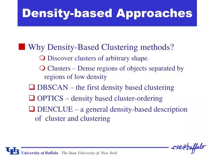
Density-based Approaches. Why Density-Based Clustering methods? Discover clusters of arbitrary shape. Clusters – Dense regions of objects separated by regions of low density DBSCAN – the first density based clustering OPTICS – density based cluster-ordering

E N D
Density-based Approaches • Why Density-Based Clustering methods? • Discover clusters of arbitrary shape. • Clusters – Dense regions of objects separated by regions of low density • DBSCAN – the first density based clustering • OPTICS – density based cluster-ordering • DENCLUE – a general density-based description of cluster and clustering
DBSCAN: Density Based Spatial Clustering of Applications with Noise • Proposed by Ester, Kriegel, Sander, and Xu (KDD96) • Relies on a density-based notion of cluster: A cluster is defined as a maximal set of density-connected points. • Discovers clusters of arbitrary shape in spatial databases with noise
Results of a k-medoid algorithm for k=4 Density-Based Clustering • Basic Idea: Clusters are dense regions in the data space, separated by regions of lower object density • Why Density-Based Clustering? Different density-based approaches exist (see Textbook & Papers)Here we discuss the ideas underlying the DBSCAN algorithm
Density Based Clustering: Basic Concept • Intuition for the formalization of the basic idea • For any point in a cluster, the local point density around that point has to exceed some threshold • The set of points from one cluster is spatially connected • Local point density at a point p defined by two parameters • e –radius for the neighborhood of point p:Ne(p) := {q in data set D | dist(p, q) e} • MinPts – minimum number of points in the given neighbourhood N(p)
-Neighborhood • -Neighborhood – Objects within a radius of from an object. • “High density” - ε-Neighborhood of an object contains at least MinPts of objects. ε-Neighborhood of p ε ε ε-Neighborhood of q p q Density of p is “high” (MinPts = 4) Density of q is “low” (MinPts = 4)
Core, Border & Outlier Outlier Given and MinPts, categorize the objects into three exclusive groups. Border • A point is a core point if it has more than a specified number of points (MinPts) within Eps These are points that are at the interior of a cluster. • A border point has fewer than MinPts within Eps, but is in the neighborhood of a core point. • A noise point is any point that is not a core point nor a border point. Core = 1unit, MinPts = 5
Example • M, P, O, and R are core objects since each is in an Eps neighborhood containing at least 3 points Minpts = 3 Eps=radius of the circles
ε ε p q Density-Reachability • Directly density-reachable • An object q is directly density-reachable from object p if p is a core object and q is in p’s -neighborhood. • q is directly density-reachable from p • p is not directly density- reachable from q? • Density-reachability is asymmetric. MinPts = 4
Density-reachability • Density-Reachable (directly and indirectly): • A point p is directly density-reachable from p2; • p2 is directly density-reachable from p1; • p1 is directly density-reachable from q; • pp2p1q form a chain. p • p is (indirectly) density-reachable from q • q is not density- reachable from p? p2 p1 q MinPts = 7
p q o Density-Connectivity • Density-reachable is not symmetric • not good enough to describe clusters • Density-Connected • A pair of points p and q are density-connected if they are commonly density-reachable from a point o. • Density-connectivity is symmetric
Formal Description of Cluster • Given a data set D, parameter and threshold MinPts. • A cluster C is a subset of objects satisfying two criteria: • Connected: p,q C: p and q are density-connected. • Maximal: p,q: if p C and q is density-reachable from p, then q C. (avoid redundancy) P is a core object.
Review of Concepts Is an object o in a cluster or an outlier? Are objects p and q in the same cluster? Are p and q density-connected? Is o a core object? Is o density-reachable by some core object? Are p and q density-reachable by some object o? Directly density-reachable Indirectly density-reachable through a chain
DBSCAN Algorithm Input: The data set D Parameter: , MinPts For each object p in D if p is a core object and not processed then C = retrieve all objects density-reachable from p mark all objects in C as processed report C as a cluster else mark p as outlier end if End For DBScan Algorithm
DBSCAN: The Algorithm • Arbitrary select a point p • Retrieve all points density-reachable from p wrt Eps and MinPts. • If p is a core point, a cluster is formed. • If p is a border point, no points are density-reachable from p and DBSCAN visits the next point of the database. • Continue the process until all of the points have been processed.
DBSCAN Algorithm: Example • Parameter • e = 2 cm • MinPts = 3 for each o Î Ddoifo is not yet classified then ifo is a core-object then collect all objects density-reachable from o and assign them to a new cluster.else assign o to NOISE
DBSCAN Algorithm: Example • Parameter • e = 2 cm • MinPts = 3 for each o Î Ddoifo is not yet classified then ifo is a core-object then collect all objects density-reachable from o and assign them to a new cluster.else assign o to NOISE
DBSCAN Algorithm: Example • Parameter • e = 2 cm • MinPts = 3 for each o Î Ddoifo is not yet classified then ifo is a core-object then collect all objects density-reachable from o and assign them to a new cluster.else assign o to NOISE
C1 MinPts = 5 P1 P C1 P C1 1. Check the -neighborhood of p; 2. If p has less than MinPts neighbors then mark p as outlier and continue with the next object 3. Otherwise mark p as processed and put all the neighbors in cluster C 1. Check the unprocessed objects in C 2. If no core object, return C 3. Otherwise, randomly pick up one core object p1, mark p1 as processed, and put all unprocessed neighbors of p1 in cluster C
C1 C1 C1 C1 C1
Example Original Points Point types: core, border and outliers = 10, MinPts = 4
Clusters When DBSCAN Works Well Original Points • Resistant to Noise • Can handle clusters of different shapes and sizes
When DBSCAN Does NOT Work Well (MinPts=4, Eps=9.92). Original Points • Cannot handle Varying densities • sensitive to parameters (MinPts=4, Eps=9.75)
Determining the Parameters e and MinPts • Cluster: Point density higher than specified by e and MinPts • Idea: use the point density of the least dense cluster in the data set as parameters – but how to determine this? • Heuristic: look at the distances to the k-nearest neighbors • Function k-distance(p): distance from p to the its k-nearest neighbor • k-distance plot: k-distances of all objects, sorted in decreasing order 3-distance(p) : p q 3-distance(q) :
Determining the Parameters e and MinPts • Example k-distance plot • Heuristic method: • Fix a value for MinPts (default: 2 d –1) • User selects “border object” o from the MinPts-distance plot;e is set to MinPts-distance(o) 3-distance first „valley“ Objects „border object“
Determining the Parameters e and MinPts • Problematic example C A F A, B, C E B, D, E G 3-Distance B‘, D‘, F, G G1 D1, D2, G1, G2, G3 G3 D G2 B D’ B’ D1 Objects D2
Density Based Clustering: Discussion • Advantages • Clusters can have arbitrary shape and size • Number of clusters is determined automatically • Can separate clusters from surrounding noise • Can be supported by spatial index structures • Disadvantages • Input parameters may be difficult to determine • In some situations very sensitive to input parameter setting
OPTICS: Ordering Points To Identify the Clustering Structure • DBSCAN • Input parameter – hard to determine. • Algorithm very sensitive to input parameters. • OPTICS – Ankerst, Breunig, Kriegel, and Sander (SIGMOD’99) • Based on DBSCAN. • Does not produce clusters explicitly. • Rather generate an ordering of data objects representing density-based clustering structure.
OPTICS con’t • Produces a special order of the database wrt its density-based clustering structure • This cluster-ordering contains info equiv to the density-based clusterings corresponding to a broad range of parameter settings • Good for both automatic and interactive cluster analysis, including finding intrinsic clustering structure • Can be represented graphically or using visualization techniques
D C C C 2 1 Density-Based Hierarchical Clustering • Observation: Dense clusters are completely contained by less dense clusters • Idea: Process objects in the “right” order and keep track of point density in their neighborhood
MinPts = 5 p e o q core-distance(o) reachability-distance(p,o) reachability-distance(q,o) Core- and Reachability Distance • Parameters: “generating” distance e, fixed value MinPts • core-distancee,MinPts(o) “smallest distance such that o is a core object”(if that distance is £e ; “?”otherwise) • reachability-distancee,MinPts(p, o) “smallest distance such that p is directly density-reachable from o”(if that distance is £e ; “?”otherwise)
OPTICS: Extension of DBSCAN • Order points by shortest reachability distance to guarantee that clusters w.r.t. higher density are finished first. (for a constant MinPts, higher density requires lower ε)
The Algorithm OPTICS • Basic data structure: controlList • Memorize shortest reachability distances seen so far (“distance of a jump to that point”) • Visit each point • Make always a shortest jump • Output: • order of points • core-distance of points • reachability-distance of points
cluster-ordered file ControlList ³ database The Algorithm OPTICS • ControlList ordered by reachability-distance. foreach o Database// initially, o.processed = false for all objects oifo.processed = false; insert (o, “?”)into ControlList; whileControlList is not empty select first element (o, r-dist) fromControlList; retrieve Ne(o) and determine c_dist= core-distance(o); set o.processed = true; write (o, r_dist, c_dist) to file; ifo is a core object at any distance £ e foreachpÎNe(o) not yet processed; determine r_distp = reachability-distance(p, o); if (p, _) ÏControlList insert (p, r_distp) in ControlList;elseif (p, old_r_dist) ÎControlListandr_distp<old_r_dist update (p, r_distp) in ControlList;
3 4 1 17 2 16 Core-distance 18 Reachability-distance OPTICS: Properties • “Flat” density-based clusters wrt. e* £ eandMinPts afterwards: • Starts with an object o where c-dist(o) £e* and r-dist(o) > e* • Continues while r-dist£e* • Performance: approx. runtime( DBSCAN(e, MinPts) ) • O( n * runtime(e-neighborhood-query) ) • without spatial index support (worst case): O( n2 ) • e.g. tree-based spatial index support: O( n* log(n) ) 1 2 17 3 16 18 4
OPTICS: The Reachability Plot • represents the density-based clustering structure • easy to analyze • independent of the dimension of the data reachability distance reachability distance cluster ordering cluster ordering
1 3 2 OPTICS: Parameter Sensitivity • Relatively insensitive to parameter settings • Good result if parameters are just“large enough” MinPts = 2, e = 10 MinPts = 10, e = 5 MinPts = 10, e = 10 1 3 2 3 1 2 2 3 1
‘ Cluster-order of the objects An Example of OPTICS neighboring objects stay close to each other in a linear sequence. Reachability-distance undefined
When OPTICS Works Well Cluster-order of the objects
When OPTICS Does NOT Work Well Cluster-order of the objects
DENCLUE: using density functions • DENsity-based CLUstEring by Hinneburg & Keim (KDD’98) • Major features • Solid mathematical foundation • Good for data sets with large amounts of noise • Allows a compact mathematical description of arbitrarily shaped clusters in high-dimensional data sets • Significantly faster than existing algorithm (faster than DBSCAN by a factor of up to 45) • But needs a large number of parameters
Denclue: Technical Essence • Model density by the notion of influence • Each data object exert influence on its neighborhood. • The influence decreases with distance • Example: • Consider each object is a radio, the closer you are to the object, the louder the noise • Key: Influence is represented by mathematical function
Denclue: Technical Essence • Influence functions: (influence of y on x, is a user given constant) • Square : f ysquare(x) = 0, if dist(x,y) > , 1, otherwise • Guassian:
Density Function • Density Definition is defined as the sum of the influence functions of all data points.
Gradient: The steepness of a slope • Example
Denclue: Technical Essence • Clusters can be determined mathematically by identifying density attractors. • Density attractors are local maximum of the overall density function.
Cluster Definition • Center-defined cluster • A subset of objects attracted by an attractor x • density(x) ≥ • Arbitrary-shape cluster • A group of center-defined clusters which are connected by a path P • For each object x on P, density(x) ≥ .