Download

1 / 55
560 likes | 711 Views
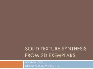
Solid Texture Synthesis from 2D Exemplars. SIGGRAPH 2007 Johannes Kopf, Chi-Wing Fu et al. Abstract. P resent a novel method for synthesizing solid textures from 2D texture exemplars Extend 2D texture optimization techniques to synthesize 3D texture solids

E N D
Solid Texture Synthesis from 2D Exemplars SIGGRAPH 2007 Johannes Kopf, Chi-Wing Fu et al.
Abstract • Present a novel method for synthesizing solid textures from 2D texture exemplars • Extend 2D texture optimization techniques to synthesize 3D texture solids • integrated with histogram matching • effectively models the material in the interior of solid objects • well-suited for synthesizing textures with a large number of channels per texel
Introduction • Solid textures have several notable advantages over 2D textures • Natural materials, such as wood and stone, may be more realistically modeled using solid textures • Solid textures obviate the need for finding a parameterization for the surface of the object to be textured • Possible to perform high-fidelity sub-surface scattering simulations, as well as break objects to pieces and cut through them
Tile-based • On-demand evaluation • Variety limited by number of tiles • Distinctive features reveal tiling structure • Cohen et al. 2003, Lefebvre et al 2003, Wei 2004 [Cohen et al. 2003] [Wei 2004] Tiles Combined to form a texture
Patch-based • Sequential • Best results • Little fine-scale variety • Praun et al 2000, Liang et al 2001,Efros and Freeman 2001, Kwatra et al 2003
Pixel-based • Fine-scale variety • Sequential • Garber 1981, Popat & Picard 1993,Efros & Leung 1999, Wei & Levoy 2000, Ashikhmin 2001, Hertzmann et al 2001, Tong et al 2002 … Exemplar Synthesized
Parallel synthesis • Most neighborhood-matching synthesis algorithms cannot support parallel evaluation • Sequential - long chains of causal dependencies • Entire image must be synthesized at one time • Cannot be mapped efficiently onto a parallel architecture like a GPU or multi-core CPU
Gen 0 (init) Gen 2 (result) Gen 1 Gen 1 Gen 2 Gen 0 Gen 0 Level 2 Level 0 Level 1 Order-independent synthesis • Wei and Levoy 2003 • Synthesize all pixels independently • Multi-scale pyramid • Apply multiple passes of correction at each pyramid level read write read write write write write write read read read read
Our method • Extend previous approach using three novel ideas • Gaussian image stack • Gaussian pyramids shifted at all locations of the exemplar image • Coordinate up-sampling • Initialize each pyramid level using coordinate inheritance • Correction sub-passes • Split each neighborhood-matching pass into several sub-passes
Our method • More explicit, intuitive control • Coordinate jitter • produces a tiling in the absence of jitter due to simple coordinate inheritance design • Set of continuous sliders that control the magnitude of random jitter • Also enables several forms of local control by adjusting spatial randomness • Synthesis magnification • Use low-res texture to synthesize a map • Use this map to efficiently sample a higher-res examplar
Basic scheme • Operate on coordinate instead of pixels • E[S[p]] = E[u] • E : Exemplar image S : Synthesized image • For exemplar image E • Create Gaussian image pyramid of total level L • S0, S1, …, (SL=S) • For exemplar image E of size m x m • L = log2m
Level 0 Level 1 Level 6 Exemplar Level 0 Level 1 Level 6 Exemplar coordinates Basic scheme
l l-1 Upsampling Jitter Correction Basic scheme • 3 fundamental steps • Up-sampling • Jitter • Correction
Up-sampling • Up-sample the coordinates of the parent pixels to its child • hl = 1 for pyramid hl = 2L-l for a stack • If jitter is disabled up-samplings create tiled image of exemplar E
(4,8) (5,8) (4,9) (5,9) (0,0) (1,0) x2 + (6,8) (7,8) (0,1) (1,1) (2,4) (3,4) (6,9) (7,9) (2,5) (8,1) (4,10) (5,10) (16,2) (17,2) (4,11) (5,11) (16,3) (17,3) Up-sampling l-1
Jitter • Perturb the up-sampled coordinates at each level • Perturb coordinates using deterministic hash function • 0 ≤ rl ≤ 1 : User-specified per-level randomness parameter • If the correction step is turned off, the effect of jitter at each level looks like a quad-tree of translated windows in the final image
Jitter Jitter Up-sampling / Jitter
Correction • Recreate neighborhoods similar to those in the exemplar • Generally perform two correction passes • For each pixel p • Match 5x5 neighborhood vector NSl(p) with NEl(u) • Consider only u in the exemplar given by 3x3 immediate neighbors of p • Pre-compute another candidate Cl1…k for exemplar pixel u • Use only one more candidate in this paper (k = 2) • For good spatial distribution each candidates are required to be separated by at least 5% of the image size • Penalize jumps to another candidate using parameter κ
Correction ? Exemplar Previous buffer (from jitter) Output Candidates { }
Traditional Gaussian image pyramid • Synthesized features align with a coarser grid • Coordinates in the synthesis pyramid are snapped to the quantized positions of the exemplar pyramid
Gaussian image stack • Allow synthesized coordinates u to have fine resolution at all levels Level 0 Level 1 Level 2 Level 3 Level 4 Level 5 Level 6 Pyramid Stack
Gaussian image stack Using Gaussian pyramid Using Gaussian Stack
Gaussian image stack • Augment the exemplar image on all sides to have size 2m×2m • Additional samples come from • Actual larger texture • Or tiling if toroidal • Or mirrored copy of exemplar • Reassign hl = 2L-l • Update up-sampling step to account for parent-child relationship
Gaussian image stack • If the exemplar is non-toroidal • Artifacts occur • When the up-sampled coordinates of four sibling pixels span over ‘mod m’ • Avoid getting boundary pixels (red in picture) as candidate Cl
Gaussian image stack • At the coarsest level (l = 0) correction step has no meaning • Stack of level 0 is equal to the mean color of the exemplar image • Correction step on stack of level 2 or below tends to restrict alignment of features • So we disable correction step on l < 3 Level 0
Correction sub-passes • Problem of traditional correction step • Pixels do not benefit from neighbors’ correction • May lead to slow convergence of pixel colors, or even to cyclic behavior • Improve results by partitioning a correction pass into a sequence of sub-passes • Apply s2 sub-passes, each one processing the pixels p such that p mod s = (i j)T, i, j ∈ {0…s-1}
Sub-passes • Nearly same amount of computation Previous buffer (from jitter) Previous buffer Subpass 1 Subpass 2 Subpass 3 Subpass 4
Sub-passes • Quality improves with more sub-passes • Not much beyond s2=9 • Traditional sequential algorithm is similar to a large number of sub-passes applied in scan-line order • Yields worse results • Gives fewer opportunities to fix earlier mistakes • On GPU, each sub-pass requires a SetRenderTarget() call, which incurs a small cost • Neighborhood error decreases with more corrections • While texture gets to look less like the exemplar due to disproportional bias cause by correction step
Spatially deterministic computation • For synthesizing a deterministic texture window Wl • Need padded window Wl′⊃ Wl • Pixels needed for padding : 2cs2 • c : number of correction step, s2 : number of sub-passes
PCA projection • 5 x 5 neighborhood of 3 dimension vector requires a lot of memory and time • Project 5 x 5 neighborhood into a lower-dimensional space • Project NEl(u) into 6 dimension vector using principal component analysis (PCA) matrix P6 • Evaluate 6 dimensional distance by these vectors
Quadrant packing • Each correction sub-pass must write to a set of nonadjacent pixels • But GPU pixel shaders do not support efficient branching on such fine granularity • Reorganize pixels according to their ‘mod s’ location
Color caching / PCA Projection of colors /Channel quantization • Fetching color information from exemplar image requires two texture lookups • Let S[p] store a tuple (u, E[u]) • (u, E[u]) is 5 dimension(channel) vector • Project this into 4 dimension vector using PCA to fit into 4 channels (RGBA) • Store most of information into 8-bit/channel textures • (Cl1(u),Cl2(u)) into RGBA texture • Projected neighborhoods ŇE(u) into 2 RGB textures • Or into 4 RGBA textures of ((Cl1(u), ŇE(Cl1(u)), Cl2(u), ŇE(Cl2(u))) • Byte sized coordinates limit exemplar size to 256 x 256
2D Hash function / GPU shader • Define a hash function using 16 x 16 2D texture • Interaction of jitter across levels helps to hide imperfections of the hash function • Hash function is only evaluated once per pixel during the jitter step • 50 x 6 Matrix P6 takes up 75 constant vector4 registers • 2D color of 5 x 5 pixels = 50 • Requires shader model ps_3_0
Multi-scale randomness control • rl set the jitter amplitude at each level • Set these parameters using a set of sliders • Coarse-scale jitter removes visible repetitive patterns at large scale
Spatial modulation • Jitter is modulated by given randomness field • Over source exemplar • By painting a randomness field RE over exemplar • Create mipmap pyramid REl[u] • Over output • By painting a randomness field RS over exemplar • Create mipmap pyramid RSl[u]
Feature drag-and-drop • Locally overrides jitter to explicitly position texture features • Constrain the synthesized coordinates in a circular region of the output • Sl[p] := (uF + (p – pF)) mod m if ||p – pF|| < rF • pF : circle center, rF: radius, uF: exemplar coordinate at pF • Must apply this constraint across many synthesis levels • Actually store two radius • Define inner radius ri, outer radius rothen interpolate across levels as rF= ril/L + ro(L-l)/L • Parameters are stored in the square cells associated with coarse image IF at resolution level is 1 • Can introduce feature variations by disabling fine scale constraint
Near-regular textures • Some textures are near-regular • Approximately periodic • Tiles may have irregular color
Near-regular textures • Given a near-regular texture image E′, resample it onto an exemplar E to be • Regular • Can be achieved using the technique of [Liu et al 2004] • determines the two translation vectors representing the underlying translational lattice and warps E′ into a “straightened” lattice • Subdivision of the unit square domain • select an nx×ny grid of lattice tiles bounded by a parallelogram and map it affinely to the unit square
Near-regular textures • Maintain tiling periodicity by quantizing each jitter coordinate • Similarly for Jl,y(p) • If local geometric distortion is desired disable quantization at fine levels • Constrain similarity set Cl(u) to the same quantized lattice (ex. ux + i(m/nx) for integer i) on levels for which hl ≥ (m/nx)
Synthesis magnification • Obtain down-sampled version of exemplar EL with some higher-resolution exemplar EH • Use synthesized coordinates SL to create higher-resolution image • Can be used to overcome 256 x 256 exemplar size limit • Very simple algorithm which can be embedded into final surface pixel shader
Synthesis magnification • Given texture coordinates p • Access the 4 nearest texels • Compute the exemplar coordinates that point p would have if it was contained in the same parametric patch • Sample the high-resolution exemplar EH at those coordinates to obtain a color • Bi-linearly blend the 4 colors
Comparison of results NVIDIA GeForce 6800 DirectX 9.0 k = 2 s2 = 4 c = 2 64 x 64 or 128 x 128 Exemplar image
Synthesis speed • GPU execution times for a 64×64 exemplar • Output is written directly into video memory, avoid the overhead of texture upload • Synthesis magnification processes 100-200 Mpixels/sec • can synthesize a 1600×1200 window by magnifying 320×240, all at 22 frames/sec
Preprocess / Representation compactness • Preprocess • Gaussian stack, PCA for colors and neighborhoods, similarity sets Cl(u) • Takes about a minute on 64 x 64 exemplar, 4-12 on 128 x 127 exemplar • Representation compactness • For 64 x 64 exemplar • Total 214KB • Minimum texture size for which the synthesis-based representation is more compact than the final image is 270×270 • For a 128×128 exemplar, it is 600×600 • May try to reduce further by compressing the representation