Download
1 / 64
640 likes | 889 Views
Intervel Estimation. 11/01/2011. A point estimate is a single value that acts as an estimate of the population parameter, interval estimation is a procedure of estimating the unknown parameter which specifies a range of values within which the parameter is expected to lie.

E N D
Intervel Estimation 11/01/2011
A point estimate is a single value that acts as an estimate of the population parameter, interval estimation is a procedure of estimating the unknown parameter which specifies a range of values within which the parameter is expected to lie.
A confidence interval is an interval computed from the sample observations x1, x2….xn, with a statement of how confident we are that the interval does contain the population parameter.
We develop the concept of interval estimation with the help of the example of the Ministry of Transport test to which all cars, irrespective of age, have to be submitted :
EXAMPLE Let us examine the case of an annual Ministry of Transport test to which all cars, irrespective of age, have to be submitted. The test looks for faulty breaks, steering, lights and suspension, and it is discovered after the first year that approximately the same number of cars have 0, 1, 2, 3, or 4 faults.
You will recall that when we drew all possible samples of size 2 from this uniformly distributed population, the sampling distribution of X was triangular:
5/25 4/25 3/25 2/25 1/25 0 0.0 0.5 1.0 1.5 2.0 2.5 3.0 3.5 4.0 Sampling Distribution ofX for n = 2
But when we considered what happened to the shape of the sampling distribution with if the sample size is increased, we found that it was somewhat like a normal distribution:
20/125 16/125 12/125 8/125 4/125 0 0.00 0.33 0.67 1.00 1.33 1.67 2.00 2.33 2.67 3.00 3.33 3.67 4.00 Sampling Distribution ofX for n = 3
And, when we increased the sample size to 4, the sampling distribution resembled a normal distribution even more closely :
100/625 80/625 60/625 40/625 20/625 0 0.00 0.25 0.50 0.75 1.00 1.25 1.50 1.75 2.00 2.25 2.50 2.75 3.00 3.25 3.50 3.75 4.00 Sampling Distribution ofX for n = 4
It is clear from the above discussion that as larger samples are taken, the shape of the sampling distribution of X undergoesdiscernible changes. In all three cases the line charts are symmetrical, but as the sample size increases, the overall configuration changed from a triangular distribution to a bell-shapeddistribution.
In other words, for large samples, we are dealing with a normal sampling distribution of . In other words:
When sampling from an infinite population such that the sample size n is large,X is normally distributed with mean and variance i.e. X is
Hence, the standardized version of X i.e. is normally distributed with mean 0 and variance 1 i.e. Z is N(0, 1).
0.4750 0.4750 0.0250 0.0250 Z -1.96 1.96 0 For the standard normal distribution, we have: The above is equivalent to P(-1.96 < Z < 1.96) = 0.4750 + 0.4750 = 0.95
0.95 0.025 0.025 Z -1.96 1.96 0
In other words: The above can be re-written as:
or or or
The above equation yields the 95% confidence interval for :
In a real-life situation, the population standard deviation is usually not known and hence it has to be estimated.
It can be mathematically proved that the quantity is an unbiased estimator of 2 (the population variance).
In this situation, the 95% Confidence Interval for is given by:
The points are called the lower and upper limits of the 95% confidence interval.
EXAMPLE-1: Consider a car assembly plant employing something over 25,000 men. In planning its future labour requirements, the management wants an estimate of the number of days lost per man each year due to illness or absenteeism. A random sample of 500 employment records shows the following situation:
Construct a 95% confidence interval for the meannumber of days lost per man each year due to illness or absenteeism.
SOLUTION 1. The point estimate of is X, which in this example comes out to be X = 5.38 days 2. In order to construct a confidence interval for , we need to compute s, which in this example comes out to be s = 3.53 days.
Hence, the 95% confidence interval for comes out to be or 5.38 0.31 days = 5.07 days to 5.69 days.
In other words, we can say that the meannumber of days lost per man each year due to illness or absenteeism lies somewhere between 5.07 days and 5.69 days, and this statement is being made on the basis of 95% confidence.
A very important point to be noted here is that we should be verycareful regarding theinterpretation of confidence intervals:
When we set 1 - = 0.95, it means that the probability is 95% that the interval will actually contain the true population mean .
In other words, if we construct a large number of intervals of this type, corresponding to the large number of samples that we can draw from any particular population, then out of every 100 such intervals, 95 will contain the true population mean whereas 5 will not.
The above statement pertains to the overall situation in repeatedsampling --- once a sample has actually been chosen from a population,X computed and the interval constructed, then this interval either contains , or does not contain .
So, the probability that our interval corresponding to sample values that have actually occurred, is either one (i.e. cent per cent), or zero. The statement 95% probability is valid before any sample has actually materialized.
In other words, we can say that our procedure of interval estimation is such that, in repeated sampling, 95% of the intervals will contain .
The above example pertained to the 95% confidence interval for .
In general, the lower and upper limits of the confidence interval for are given by Where the value of z/2 depends on how much confidence we want to have in our interval estimate.
Z 0 The above situation leads to the (1-) 100% C.I. for .
If (1-) = 0.95, then z/2 = 1.96 whereas If (1-) = 0.99, then z/2 = 2.58 and If (1-) = 0.90, then z/2 = 1.645 . (The above values of z/2 are easily obtained from the area table of the standard normal distribution).
An important to note is that, as indicated earlier, the above formula for the conference interval is valid when we are sampling from an infinite population in such a way that the sample size n is large.
Howlarge should n be in a practical situation? The rule of thumb in this regard is that whenever n 30, we can use the above formula.
Confidence Interval for ,the Mean of an Infinite Population: For large n (n 30), the confidence interval is given by where is the sample mean and is the sample standard deviation.
Let us consolidate the idea by looking at a few moreexamples:
EXAMPLE-1 The Punjab Highway Department is studying the traffic pattern on the G.T. Road near Lahore. As part of the study, the department needs to estimate the average number of vehicles that pass the Ravi bridge each day.
A random sample of 64 days gives X = 5410 and s = 680. Find the 90 per cent confidence interval estimate for , the average number of vehicles per day.