Download
1 / 28
340 likes | 674 Views
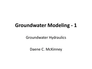
Groundwater Modeling – 2: Computer Implementation. Groundwater Hydraulics Daene C. McKinney. Groundwater Vistas. Groundwater Modeling Environment Graphic User Interface (GUI) for MODFLOW and other models Imports a wide variety of files MODFLOW data sets ArcView shapefiles

E N D
Groundwater Modeling – 2:Computer Implementation Groundwater Hydraulics Daene C. McKinney
Groundwater Vistas • Groundwater Modeling Environment • Graphic User Interface (GUI) for MODFLOW and other models • Imports a wide variety of files • MODFLOW data sets • ArcViewshapefiles • Digitized map files (AutoCAD DXF, Shapefiles, and SURFER) • GroundwaterVistas is not MODFLOW (but includes it) • MODFLOW has no Graphic User Interface (GUI)
Groundwater Vistas Installation • Download file: gv5final.zip from • http://www.caee.utexas.edu/prof/mckinney/ce374l/Overheads/gv5final.zip • Unzip gv5final.zip to get • gv5final.exe (a “setup” file) • Run gv5final.exe to install • Groundwater Vistas version 5 • Answer “yes” or “OK” to everything • Groundwater Vistas manuals installed in • C:\gwv5\manuals
Unit System • Use a consistent set of units for all data • Select a unit of length and time • Hydraulic conductivity (K) in m/s • Pumping rates (Q) in m3/s • Length units in m • Elevations in m
Example Pumping Well Layer 1 10 m 13 • Boundaries • North & South: No-flow • East & West: Constant-head • Layer 1 – unconfined (13 m) • Kh = 5x10⁻³ m/s • Kv = 5x10⁻⁴ m/s • Layer 2 – confined (5 m) • Kh = 1x10⁻³ m/s; Kv = 1x10⁻⁴ m/s Layer 2 -3 m 5 -8 m No-flow Boundary N Pumping Well Constant Head Boundary (h = 9 m) Constant Head Boundary (h = 8 m) 600 m No-flow Boundary Adapted from Chiang, W-H and W. Kinzelbach, Processing Modflow: A Simulation System For Modeling Groundwater Flow and Pollution, 1996 600 m
Create a New Model • Start the GV program • Select File New
Create a New Model • Enter basic information • 30 rows • 30 columns • Row spacing = 20 m • Column spacing = 20 m • Top of Layer 1 = 10 m • Bottom of Layer 1 = -3 m • Bottom of Layer 2 = -8 m Press
Model Grid Elevation = +10 m Elevation = -3 m Elevation = -8
Add Constant Head Boundary Conditions • Select: Layer 1 • Select: BCs Constant Head Boundary • Select: BCs Insert Window • Hold left Mouse button and Drag cursor through cells in Column 1 • Set value to 9 m Constant Head Boundary Cells (h = 9 m) Press OK Top Layer - 1
Repeat for Boundary in Column 30 • Select: Layer 1 • Select: BCs Constant Head Boundary • Select: BCs Insert Window • Hold left Mouse button and Drag cursor through cells in Column 30 • Set value to 8 m Constant Head Boundary Cells (h = 8 m) Top Layer - 1
Repeat for Layer 2 • Select: Layer 2 • Select: BCs Constant Head Boundary • Select: BCs Insert Window • Hold left Mouse button and Drag cursor through cells in Columns 1 and 30 • Set values to 9 and 8 m Constant Head Boundary Cells (h = 8 m) Bottom Layer - 2
Add Hydraulic Conductivity • Select: Props Hydraulic Conductivity • Select: Property Values Database • Set up 2 zones: • Layer 1 • Kx = 5x10⁻³ m/s • Ky= 5x10⁻³ m/s • Kz = 5x10⁻⁴ m/s • Layer 2 • Kx= 1x10⁻³ m/s • Ky= 1x10⁻³ m/s • Kz = 1x10⁻⁴ m/s • Click OK
Assign K to Layer 1 • Select: Layer 1 • Select: Props Hydraulic Conductivity • Select: Props Set Value or Zone Window • Start in upper right-hand corner and drag to select all cells in grid • Select: OK • Select: Zone Number 1 • Select: OK
Assign K to Layer 2 • Select: Layer 2 • Select: Props Hydraulic Conductivity • Select: Props Set Value or Zone Window • Start in upper right-hand corner and drag to select all cells in grid • Select: OK • Select: Zone Number 2 • Select: OK
Add Multi-Layer Well Pumping Well Layer 1 • Well penetrates all layers • Total pumping rate for multilayer well is sum of pumping from layers • Pumping for each layer (Qk) is proportional to layer transmissivity (bK) • For a total pumping rate of Qtotal= 0.02 m3/s • Q1 = 0.0185 m3/s • Q2 = 0.0015 m3/s Layer 2
Add Well in Layer 1 • Select: Layer 1 • Select: BCs Well • Select: BCs Insert Single Cell • Use cursor to click on cell at Row 15, Col. 25 • Enter “Flow Rate in Well” = - 0.0185 m3/s • Select: OK Row 15, Column 25 Note Top Layer - 1
Add Well in Layer 2 • Select: Layer 2 • Select: BCs Well • Select: BCs Insert Single Cell • Use cursor to click on cell at Row 15, Col. 25 • Enter “Flow Rate in Well” = - 0.0015 m3/s • Select: OK Row 15, Column 25 Note Top Layer - 1
Create MODFLOW Dataset • Select: Model MODFLOW Package Options • Select: Time Units = seconds • Select: Length Units = meters
Create MODFLOW Dataset • Select: Model MODFLOW Package Options • Select: Tab Initial Heads • Enter: 0 ft for both Layers
Create MODFLOW Dataset • Select: Model MODFLOW Package Options • Select: Tab BCF-LPF • Select: Layer 1 as “Unconfined” • Select: Layer 2 as “Confined”
Create MODFLOW Dataset • Select: Model MODFLOW Package Options • Select: Tab Recharge - ET • Select: Top Layer Only • Select: OK
Run Simulation • Select: Calculator button • Select: Yes, Yes, Yes!
Process Results • Select: Cell-by-cell flows
Results • Select: Plot Contour Parameters (Plan) • Set parameters to achieve the display you like
Set Display Options • Select: Plot What to display • Select: Display Color Flood of Head • Select: Display Legend • Select: OK
Set Legend Options • Select: Plot Legend Options • Select: Contents • Select: Color Flood Scale • Select: Dry Cells • Select: Title • Select: Title Font = 10 bold • Select: Text Font = 10 • Select: OK
Results • Look for the file ‘Ex1.lst” in the directory that you specified for the “working directory” (e.g., C:\gv5\models). • Look for the following table and make sure you get the same (or close) numbers