Download
1 / 29
300 likes | 499 Views
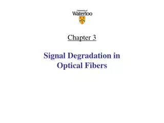
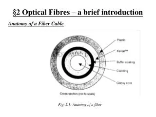
§2 Optical Fibres – a brief introduction. Anatomy of a Fiber Cable. Fig. 2.1: Anatomy of a fiber. Index of Refraction Profiles. Fig. 2.2: Step index and graded index profiles in fiber. Critical Cone or Acceptance Cone

E N D
§2 Optical Fibres – a brief introduction Anatomy of a Fiber Cable Fig. 2.1: Anatomy of a fiber
Index of Refraction Profiles Fig. 2.2: Step index and graded index profiles in fiber.
Critical Cone or Acceptance Cone Critical cone, also known as acceptance cone, is a cone of an angle within which all rays that are launched into the core are reflected at the core-cladding interface at or beyond the critical angle (Fig. 3.6). The half angle of the critical cone, also know as numerical aperture, depends on the refractive index distribution function in the core and cladding, and is independent of the core diameter. For a step-index fiber, the numerical aperture is where n1 is for the core and n2 for the cladding. Fig. 2.3: Illustrative definition of critical cone.
Phase Velocity A monochromatic wave (single or ) that travels along the fiber axis is described by where E is the amplitude of the field, = 2f, and is the propagation constant. Phase velocity, V, is defined as the velocity of an observer that maintains constant phase with the traveling field, that is, t - x = constant. Replacing the traveled distance x within time t, x = V t, then the phase velocity of the monochromatic light in the medium is
Group Velocity A modulated optical signal contains frequency components that travel (in the fiber) with slightly different phase velocities. This is explained mathematically as follows. Consider an amplitude-modulated optical signal traveling along the fiber: where E is the electric field, m is the modulation depth, is the modulation frequency, c is the frequency of light (or carrier frequency), and c. Trigonometric expansion of the above expression results in three frequency components with arguments c, c , and c +
Each component travels along the fiber at a slightly different phase velocity (c, c , c + , respectively) occurring a different phase shift. Eventually, all three components form a spreading envelope that travels along the fiber with a phase velocity: Group velocity, (g = c/ng), is defined as the velocity of an observer that maintains constant phase with the group traveling envelope; that is, t () x = constant. Replacing x by gt, then, the group velocity is expressed by g=/ = / = 1/ where is the propagation constant, and is the first partial derivative w.r.t. . Group velocity is particularly significant in optical data transmission where light is modulated.
Fiber Modes Fig. 2.4: Multimode and single-mode fiber cross-section The number of modes a fiber can support is determined by the refractive index profile, the operating light wavelength and the core size.
Theories of light propagation in a fibre 1. Ray theory – gives an intuitive feel for light containment and light pulse spreading. It is accurate for multimode fibres. 2.Wave theory – useful in explaining absorption, attenuation and dispersion. Accurate in all cases, especially in explaining single mode fibres, coherence phenomena, field distribution of modes, bending loss.
Ray theory Fibre Mode: Set of guided lightwaves which propagates inside the fibre. Fig. Comparison of single-mode and multimode step-index and graded-index optical fibers.
Wave (Field) Analysis The wave analysis starts with Maxwell’s wave equation for the electric field: . Wave equation for magnetic field: The light field that propagates in a step index fibre is the solution of the above two equations with appropriate boundary conditions. It has been proved that the solution for of the equation can be decomposed to a discrete series of modes, i.e.,
Each term (mode) in the expansion much itself be a solution of the equations. LPlm modes: LP: “linearly polarized”. The accuracy of the LP mode designation is good in the weakly guiding approximation (i.e., <<1). In the weakly guiding approximation, the z-component of Ei(x,y)or Ei(r,) is very small and can be practically neglected. Ei(x,y)or Ei(r,) will only have transverse components that can be decomposed to an x-component and a y-component, corresponding two linearly polarized light components. The value of l is one-half the number of minima (or maxima) that occur in the intensity patter as varies through 2 radians; m is the number of maxima in the intensity pattern that occur along a radial line between zero and infinity.
(a) (a) (b) (b) Fig. 2.5: Intensity plots for the LP modes, with a = 1. (a) LP01; (b) LP11;
(c) (c) (d) (d) Fig. 2.5: Intensity plots for the six LP modes, with a = 1. (c) LP21; (d) LP02
(e) (e) (f) (f) Fig. 2.5: Intensity plots for the six LP modes, with a = 1. (e) LP31; (f) LP12;
The V number: An important parameter connected with the cut-off condition of modes is the normalized frequency V (also called V number or V parameter) defined by The larger the V number, the more modes a fiber can support. The number of modes M supported by a multi mode fiber is For V<2.405, only one mode, i.e., the LP01 mode, is supported; other modes cannot propagate within the fiber. We say the fiber is a single mode (SM) fiber.
Cut-off wavelength For a fixed fiber, if the light wavelength is smaller, V number will be bigger. This implies that a single mode fiber at a longer wavelength (i.e., 1550nm) could support more than one mode at shorter wavelength (say 633 nm). The critical wavelength corresponding to the second mode to leak is called cut-off wavelength of the fiber, defined as The cut-off wavelength is usually specified by the fiber manufacture. When the working wavelength is longer than the cut-off wavelength, the fiber is single-mode, otherwise it will be multi-mode.
Mode Field Distribution of SM fiber The mode filed distribution of a single mode fiber is also affected by the V number. The larger the V number, the more light power in the fiber core, less optical power in the cladding. The Mode Field Diameter (MFD) is inversely proportional to the V number.
Polarization in SM fiber Birefringence: Beat Length:
Dispersion in optical fibers ●A pulse propagating in fiber is broaden with amplitude reduced, Why? ●Fibre dispersion causes pulses to be broaden (i) Intermoal (or modal) dispersion (ii) Intramodal (or chromatic) disperaion ●Pulse spread causes ISI and hence affect the performance of the communication systems
Modal Dispersion ●An input pulse excites a number of modes (rays) ●Different modes travels at different speeds and experiences different delays, causing pulse to spread ●The unit of modal dispersion is ps/km
Chromatic dispersion - physics Chromatic dispersion: for the same mode, e.g., LP01 mode, different wavelength components travel at different speed. Unit: ps/(km.nm) Chromatic dispersion consists of two contributions: material dispersion and waveguide dispersion Material dispersion: refractive index ands hence the speed of light in materials are wavelength dependent Waveguide dispersion: the power distribution in the core/cladding and hence the effect index are wavelength dependent
Polarization mode dispersion DPMD is the average PMD parameter and is measured in Typical values of DPMD range from 0.1 to 1.0 PMD is critical for high-rate long-haul links that are designed to operate near the zero-dispersion wavelength of the fiber.
Questions • Which effect is bigger in multi mode fiber optic communication systems, modal dispersion or chromatic dispersion? • In single mode fiber, modal dispersion is zero, true or false? • PMD is not important for short distance communication systems, why?
Fiber attenuation or loss Fiber attenuation coefficient or constant: = [1/L]10log[P(0)/P(L)] = -[10/L]log[P(L)/P(0)] or P(L) = P(0) 10L10 where P(0) and P(L) are respectively the launched power into the fiber and output power at a length L. If we replace P(L) with Pr, the minimum acceptable power at the receiver, then the (ideal) maximum fiber length is Lmax = [10/ ] log10[P(0)Pr] ●Fibre loss reduces the amplitude of signal and limits the repeaterless fiber span ● Question: What are the other factors that limit the maximum fiber length?
Fig. Typical single-mode fiber attenuation graph. The LUCENT Technologies AllWave fiber has eliminated losses due to OH (dotted line). Fiber attenuation or loss depends on the wavelength: = C1 / 4 + C2 + A(4.19) where C1 is a constant due to Rayleigh scattering, C2 is a constant due to fiber imperfections, and A() is a function that describes the absorption of wavelengths by impurities in the fiber. Unit: dB/km Typical values: 0.4dB/km at 1310nm. 0.2dB/km at 1550nm. Ordinary glass: 1dB/cm
The decibel The power can also be expressed in terms of dBm. The dBm is defined with respect to a reference level of 1mW, as 10log(P/1mW) (dBm) For example, a power level of 1mW and 1μW correspond respectively to 0dBm and -30dBm. With the definition of dBm, the net power loss (in dB) of a fiber or a fiber component can be easily calculated as the input power in dBm – the output power in dBm. Example: 2mW (or 3dBm) power is launched into a fiber of 20km, the output power is -10dBm (or 0.1mW). The power loss of the fiber is 3dBm-(-10dBm)=13dB. The fiber attenuation coefficient is 13dB/20km = 0.65dB/km.
Fiber-to-fiber joints • Low loss Interconnections are needed • between a source and a fiber • between a fiber and a photodetector • Between two fibers • A splice is a permanent bound between fibers • A connector is a demountable joint between fibers • Mechanical alignment • Fiber end-face preparation • Fiber splicing • Fiber connectors
Fibre materials: ● Silica glass fibers ● Halide glass fibers ● Active glass fibers (rare-earth doped) ● Plastic fibers