Download
1 / 21
210 likes | 294 Views
Explore the fundamentals of neural networks with a focus on Perceptrons and Gradient Descent algorithms. Learn how these models work, the training processes involved, and their applications in pattern recognition and decision-making.

E N D
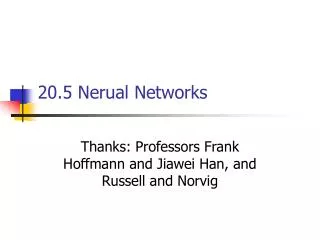
20.5 Nerual Networks Thanks: Professors Frank Hoffmann and Jiawei Han, and Russell and Norvig
Biological Neural Systems • Neuron switching time : > 10-3 secs • Number of neurons in the human brain: ~1010 • Connections (synapses) per neuron : ~104–105 • Face recognition : 0.1 secs • High degree of distributed and parallel computation • Highly fault tolerent • Highly efficient • Learning is key
A Neuron ak Wkj • Computation: • input signals input function(linear) activation function(nonlinear) output signal output inj aj Input links output links å ai = output(inj) j
x1 x2 xn Part 1. Perceptrons: Simple NN inputs weights w1 output activation w2 y . . . q a=i=1n wi xi wn Xi’s range: [0, 1] 1 if a q y= 0 if a< q {
Decision Surface of a Perceptron 1 1 Decision line w1 x1 + w2 x2 = q x2 w 1 0 0 0 x1 1 0 0
Linear Separability x2 w1=? w2=? q= ? w1=1 w2=1 q=1.5 0 1 0 1 x1 x1 1 0 0 0 Logical XOR Logical AND
x1 x2 xn Threshold as Weight: W0 q=w0 1 if a 0 y= 0 if a<0 x0=-1 w1 w0 w2 y . . . a= i=0n wi xi wn {
Training the Perceptron p742 • Training set S of examples {x,t} • x is an input vector and • t the desired target vector • Example: Logical And S = {(0,0),0}, {(0,1),0}, {(1,0),0}, {(1,1),1} • Iterative process • Present a training example x , compute network output y , compare output y with target t, adjust weights and thresholds • Learning rule • Specifies how to change the weights w and thresholds q of the network as a function of the inputs x, output y and target t.
Perceptron Learning Rule • w’=w + a (t-y) x wi := wi + Dwi = wi + a (t-y) xi (i=1..n) • The parameter a is called the learning rate. • In Han’s book it is lower case L • It determines the magnitude of weight updates Dwi . • If the output is correct (t=y) the weights are not changed (Dwi =0). • If the output is incorrect (t y) the weights wi are changed such that the output of the Perceptron for the new weights w’i is closer/further to the input xi.
Perceptron Training Algorithm Repeat for each training vector pair (x,t) evaluate the output y when x is the input if yt then form a new weight vector w’ according to w’=w + a (t-y) x else do nothing end if end for Until y=t for all training vector pairs or # iterations > k
Perceptron Convergence Theorem • The algorithm converges to the correct classification • if the training data is linearly separable • and learning rate is sufficiently small • If two classes of vectors X1 and X2 are linearly separable, the application of the perceptron training algorithm will eventually result in a weight vector w0, such that w0 defines a Perceptron whose decision hyper-plane separates X1 and X2 (Rosenblatt 1962). • Solution w0 is not unique, since if w0 x =0 defines a hyper-plane, so does w’0= k w0.
x1 x2 xn Perceptron Learning from Patterns w1 w2 . . . wn weights (trained) fixed Input pattern Association units Summation Threshold Association units (A-units) can be assigned arbitrary Boolean functions of the input pattern.
Part 2. Multi Layer Networks Output vector Output nodes Hidden nodes Input nodes Input vector
Gradient Descent Learning Rule • Consider linear unit without threshold and continuous output o (not just –1,1) • Output=oj=-w0 + w1 x1 + … + wn xn • Train the wi’s such that they minimize the squared error • Error[w1,…,wn] = ½ jD (Tj-oj)2 where D is the set of training examples
x1 x2 xn Neuron with Sigmoid-Function inputs weights w1 output activation w2 o . . . a=i=1n wi xi wn Output=o=s(a) =1/(1+e-a)
x1 x2 xn Sigmoid Unit x0=-1 w1 w0 a=i=0n wi xi o=(a)=1/(1+e-a) w2 o . . . (x) is the sigmoid function: 1/(1+e-x) wn d(x)/dx= (x) (1- (x)) • Derive gradient decent rules to train: • one sigmoid function • E/wi = -j(Tj-O) o(1-o) xij • derivation: see next page
Explantion: Gradient Descent Learning Rule yj wi = a Ojp(1-Ojp) (Tjp-Ojp) xip wji xi activation of pre-synaptic neuron learning rate error djof post-synaptic neuron derivative of activation function
(w1,w2) (w1+w1,w2 +w2) Gradient Descent: Graphical D={<(1,1),1>,<(-1,-1),1>, <(1,-1),-1>,<(-1,1),-1>}
Perceptron vs. Gradient Descent Rule • Perceptron rule w’i = wi + a (t-o) xi derived from manipulation of decision surface. • Gradient descent rule w’i = wi + a (1-y) (t-y) xi derived from minimization of error function E[w1,…,wn] = ½ p (t-y)2 by means of gradient descent.