Download
1 / 10
110 likes | 358 Views
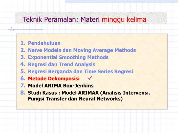
Teknik Peramalan: Materi minggu kelima. Pendahuluan Naïve Models dan Moving Average Methods Exponential Smoothing Methods Regresi dan Trend Analysis Regresi Berganda dan Time Series Regresi Metode Dekomposisi Model ARIMA Box-Jenkins

E N D
Teknik Peramalan: Materi minggu kelima • Pendahuluan • Naïve Models dan Moving Average Methods • Exponential Smoothing Methods • Regresi dan Trend Analysis • Regresi Berganda dan Time Series Regresi • Metode Dekomposisi • Model ARIMA Box-Jenkins • Studi Kasus : Model ARIMAX (Analisis Intervensi, Fungsi Transfer dan Neural Networks)
Kaitan Pola Data dan Metode Dekomposisi Dekomposisi Adititif (Trend & Seasonal) Constant Variation Dekomposisi Multiplikatif (Trend & Seasonal) Unconstant Variation
Model Dekomposisi MULTIPLIKATIF Bentuk umumModel dekomposisi multiplikatif Yt= Tt St Ct It dengan : Yt = Nilai pengamatan waktu ke-t Tt = Komponen (faktor) trend waktu ke-t St = Komponen (faktor) musim waktu ke-t Ct = Komponen (faktor) siklus waktu ke-t It = Komponen (faktor) irregular waktu ke-t
How MINITAB Does Decomposition (multiplicative) 1. Minitab fits a trend line to the data, using least squares regression. 2. Next, the data are detrended by dividing the data by the trend component. 3. Then, the detrended data are smoothed using a centered moving average with a length equal to the length of the seasonal cycle. When the seasonal cycle length is an even number, a two-step moving average is required to synchronize the moving average correctly. 4. Once the moving average is obtained, it is divided into the detrended data to obtain what are often referred to as raw seasonals. 5. Within each seasonal period, the median value of the raw seasonals is found. The medians are also adjusted so that their mean is one. These adjusted medians constitute the seasonal indices. 6. The seasonal indices are used in turn to seasonally adjust the data.
Data jumlah pesanan minuman “ABC” (ribu unit)(Bowerman & O’Connel)
MINITAB output: Data pesanan “ABC” (Bowerman & O’Connel)