Download
1 / 24
240 likes | 411 Views
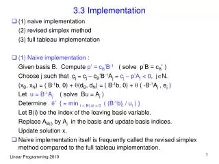
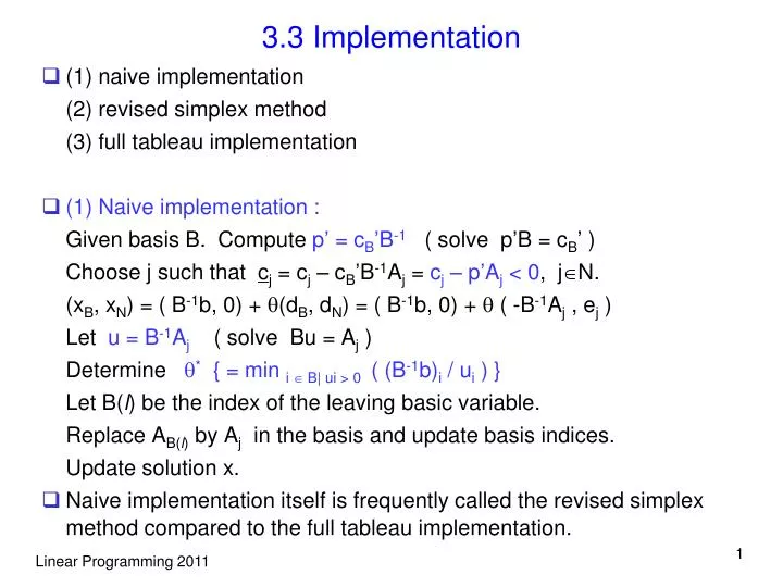
3.3 Implementation. (1) naive implementation (2) revised simplex method (3) full tableau implementation (1) Naive implementation : Given basis B. Compute p’ = c B ’B -1 ( solve p’B = c B ’ ) Choose j such that c j = c j – c B ’B -1 A j = c j – p’A j < 0 , j N.

E N D
3.3 Implementation • (1) naive implementation (2) revised simplex method (3) full tableau implementation • (1) Naive implementation : Given basis B. Compute p’ = cB’B-1 ( solve p’B = cB’ ) Choose j such that cj = cj – cB’B-1Aj = cj – p’Aj < 0, jN. (xB, xN) = ( B-1b, 0) + (dB, dN) = ( B-1b, 0) + ( -B-1Aj , ej ) Let u = B-1Aj ( solve Bu = Aj ) Determine * { = min i B| ui > 0 ( (B-1b)i / ui ) } Let B(l) be the index of the leaving basic variable. Replace AB(l) by Aj in the basis and update basis indices. Update solution x. • Naive implementation itself is frequently called the revised simplex method compared to the full tableau implementation.
(2) Revised simplex method : Naive implementation needs to find p’ = cB’B-1 and u = B-1Aj ( or solve p’B = cB’, Bu = Aj ) in each iteration. Update B-1 efficiently so that computational burden is reduced. (compute cB’B-1 and B-1Aj easily. Similar idea can be used to update B efficiently and find p, u vectors easily.) • B = [ AB(1), … , AB(m) ] B = [ AB(1), .., AB(l-1) , Aj , AB(l+1) ,.. , AB(m) ] B-1B = [ e1 , … , el-1 , u , el+1 , … , em ], u = B-1Aj Premultiply elementary row operation matrices QkQk-1 … Q1 Q to B-1B so that Q B-1B = Q [ e1 , … , el-1 , u , el+1 , … , em ] = I QB-1 = B-1 Hence applying the same row operations ( to convert u to el ) to B-1 results in B-1. ( see example in the text)
(3) Full tableau implementation : Ax = b B-1Ax = B-1b maintain [ B-1b : B-1A1 , … , B-1An ] can read current b.f.s. x from B-1b and dB = -B-1Aj Update to B-1 [ b : A ]. We know B-1 = QB-1 Hence B-1 [ b : A ] = QB-1 [ b : A ] = Q [B-1b : B-1A ] So apply row operations, which convert u = B-1Aj to el , to the matrix [B-1b : B-1A ] (To find exiting column AB(l) and step size *, compare xB(i)/ui for ui > 0, i = 1, … , m. ) Also maintain and update information about reduced costs and objective value.
To update the 0-th row, add k (pivot row) to 0-th row for some scalar k so that the coefficient for the entering variable xj in 0-th row becomes 0. Currently 0-th row is [ 0 : c’ ] – g’ [ b : A ] , where g’ = cB’B-1. Let column j be the pivot column and row l be the pivot row. Pivot row l of [ B-1b : B-1A ] is h’ [ b : A ] where h’ is l-th row of B-1. Hence, after adding, new 0-th row still represented as [ 0 : c’ ] – p’ [ b : A] for some p, while cB(l) – p’AB(l) = cj –p’Aj = 0
(continued) Now for xi basic, i l, have ci remains at 0. ( ci = 0 before the pivot. Have B-1AB(i) = ei , i l. Hence (B-1AB(i))l = 0 ) cB(i) - p’AB(i) = 0, for all i B cB’ – p’B = 0 p’ = cB’B-1 new 0-th row is [ 0 : c’ ] – cB’B-1 [ b : A ] as desired.
Ex: x4 = x5 = x6 = x4 = x1 = x6 =
(Remark) (1) Tableau form also can be derived as the following : Given min c’x, Ax = b, x 0, let A = [ B : N ], x = [ xB , xN ], c = [ cB , cN ], where B is the current basis. Also let z denote the value of the objective function, i. e. z = c’x. Since all feasible solutions must satisfy Ax = b, they must satisfy [ B : N ] [ xB , xN ]’ = b BxB + NxN = b BxB = b – NxN xB = B-1b – B-1NxN ( IxB + B-1NxN = B-1b ) or in matrix form, [ I : B-1N ] [ xB , xN ]’ = B-1b
(continued) Since all feasible solutions must satisfy these equations, we can plug in the expression for xB into the objective function to obtain z = c’x = cB’xB + cN’xN = cB’ (B-1b – B-1NxN) + cN’xN = cB’ B-1b + 0’xB + ( cN’ - cB’ B-1N) xN = cB’ B-1b + ( cN’ – p’N) xN , where p’ = cB’ B-1 or p’B = cB’ Hence obtain the tableau with respect to the current basis B z - cB’ B-1b = 0’xB + ( cN’ - cB’ B-1N) xN B-1b = I xB + B-1N xN ( =(B-1A)x ) See text for an example of full tableau implementation.
(continued) (2) Tableau also can be obtained using the following logic. Note that elementary row operations on equations do not change the solution space, but the representation is changed. Starting from -z + cB’xB + cN’xN = 0 BxB + NxN = b We compute multiplier vector y for the constraints by solving y’B = cB’ ( y’ = cB’B-1). Then we take linear combination of constraints using weight vector –y and add it to objective row, resulting in -z + 0’xB + ( cN’ - cB’ B-1N) xN = - cB’ B-1b. We multiply B-1 on both sides of constraints I xB + B-1N xN = B-1b
Practical Performance Enhancements • In commercial LP solver, B-1 is not updated in the revised simplex method. Instead we update the representation of B as B = LU, where L is lower triangular and U is upper triangular matrices (with some row permutation allowed, LU decomposition, triangular factorization). • We solve the system (with proper updates), p’LU = cB’, LUu = Aj, each system takes O(m2) to solve and numerically more stable than using B-1. Moreover, less fill-in occurs in LU decomposition than in B-1, which is important when we solve large sparse problems.
3.4 Anticycling • 1. Lexicographic pivoting rule • Def : u Rn is said to be lexicographically larger than v Rn if u v and the first nonzero component of u – v is positive ( u > v ) • Lexicographic pivoting rule (1) choose entering xj with cj < 0. Compute updated column u = B-1Aj . (2) For each i with ui > 0, divide i-th row of the tableau by ui and choose lexicographically smallest row. If row l is smallest, xB(l) leaves basis. (see example in the text)
Ex: Suppose pivot column is the third one ( j = 3) ratio = 1/3 for 1st and 3rd row third row is pivot row, and xB(3) exits the basis.
Thm : Suppose the rows in the current simplex tableau is lexicographically positive except 0-th row and lexicographic rule is used, then (a) every row except 0-th remains lexicographically positive. (b) 0-th row strictly increases lexicographically. (c) simplex method terminates finitely.
Pf) (a) Suppose xj enter, xlleaves ( ul > 0 ) Then ( l-th row ) / ul < ( i-th row ) / ui , i l , ui > 0 ( l-th row ) ( l-th row ) / ul ( lexicographically positive ) For i-th row, i l (1) ui < 0 ; add pos. num. ( l-th row ) to i-th row lex. pos. (2) ui > 0 ; (new i-th row) = (old i-th row) – ( ui / ul )(old l-th row) lexicographically positive (3) ui = 0 ; remain unchanged (b)cj < 0 we add positive multiple of l-th row to 0-th row (c) 0-th row determined by current basis no basis repeated since 0-th row increases lexicographically finite termination.
Remarks : (1) To have initial lexicographically positive rows, permute the columns (variables) so that the basic variables come first in the current tableau (2) Idea of lexicographic rule is related to the perturbation method. If no degenerate solution objective value strictly decreases, hence no cycling. Hence add small positive i to xB(i) , i = 1, … , m to obtain xB(i) = (B-1b)i + i , where 0 < m << m-1 << … << 2 <<1 <<1
(continued) It can be shown that no degenerate solution appears in subsequent iterations ( think I’s as symbols), hence cycling is avoided. Lexicographic rule is an implementation of the perturbation method without using i’s explicitly. Note that the coefficient matrix of i’s and basic variables are all identity matrices. Hence the simplex iterations (elementary row operations) results in the same coefficient matrices.
2. Bland’s rule ( smallest subscript rule ) (1) Find smallest j for which cj < 0 and have the column Aj enter the basis (2) Out of all variables xi that are tied in the test for choosing an exiting variable, choose the one with the smallest value of i. Pf) see Vasek Chvatal, Linear Programming, Freeman, 1983 • Note that the lexicographic rule and the Bland’s rule can be adopted and stopped at any time during the simplex iterations.
3.5 Finding an initial b.f.s. • Given (P): min c’x, s.t. Ax = b, x 0 ( b 0 ) Introduce artificial variables and solve (P-I) min y1 + y2 + … + ym , s.t. Ax + Iy = b, x 0, y 0 Initial b.f.s. : x = 0, y = b If optimal value > 0 (P) infeasible (If P feasible P-I has solution with y = 0 ) If optimal value = 0 all yi = 0, so current optimal solution x gives a feasible solution to (P). Drop yi variables and use original objective function. However, we need a b.f.s. to use simplex. Have trouble if some artificial variables remain basic in the optimal basis.
Driving artificial variables out of the basis Pivot element
Suppose { xB(1), … , xB(k) } , k < m are basic variables which are from original variables. Suppose artificial variable yi is in the l-th position of the basis ( l-th component of the column for yi in the optimal tableau is 1 and all other components are 0. ) and l-th component of B-1Aj is nonzero for some nonbasic original variable xj. Then { B-1AB(1) , … , B-1AB(k) } = { e1, ... , ek } and B-1Aj linearly independent { AB(1) , … , AB(k) , Aj } linearly independent So bring xj into the basis by pivoting (solution not changed) • If not exist xj with (B-1Aj)l 0 g’A = 0’ (g’ is l-th row of B-1) So rows of A linearly dependent. Also have g’b = 0 since Ax = b feasible. Hence g’Ax = g’b ( 0’x = 0’ ) redundant eq. and it is l-th row of tableau eliminate it.
Remarks • Note that although we may eliminate the l-th row of the current tableau, it may not imply that the l-th row of the original tableau is redundant. To see this, suppose that i-th artificial variable (with corresponding column ei in the initial tableau) is in the l-th position of the current basis matrix (hence B-1ei = el in the current tableau). Let g be the l-th row of B-1 , then from g’ei = 1, we know that i-th component of g is 1. Then, from g’A = 0’ and g’b = 0, i-th row of [b : A] can be expressed as a linear combination of the other rows, hence i-th row in the original tableau is redundant.
Sometimes, we may want to retain the redundant rows when we solve the problem because we do not want to change the problem data so that we can perform sensitivity analysis later, i.e. change the data a little bit and solve the problem again. Then the artificial variables corresponding to the redundant equations should remain in the basis (we should not drop the variable). It will not leave the basis in subsequent iterations since the corresponding row has all 0 coefficients. • If we do not drive the artificial variables out of the basis and perform the simplex iterations using the current b.f.s., it may happen that the value of the basic artificial variables become positive, hence gives an infeasible solution to the original problem. To avoid this, modification on the simplex method is needed or we may use the bounded variable simplex method by setting the upper bounds of the remaining artificial variables to 0. ( lower bounds are 0 )
Two-phase simplex method • See text p116 for two-phase simplex method • Big-M method Use the objective function min , where M is a large number. • see text sec. 3.6 for definition of k-dimensional simplex and the interpretation of simplex method by column geometry.
3.7 Computational efficiency of the simplex method • Each iteration of the simplex method takes polynomial time of m, n and length of encoding of data. But number of iterations is exponential in the worst case/ Empirically, number of iterations is O(m) and O(log n). For pivoting rules, there exist counter examples on which simplex takes exponential number of iterations, hence simplex algorithm is not a polynomial time algorithm. ( Still, there exists a possibility that some other pivoting rules may provide polynomial running time. Though it may be very difficult to prove.)