Download

1 / 28
280 likes | 391 Views
Linear-Time Reconstruction of Zero-Recombinant Mendelian Inheritance on Pedigrees without Mating Loops. Authors: Lan Liu , Tao Jiang Univ. California, Riverside USA ,. Outline. Introduction and problem definition The linear system for ZRHC

E N D
Linear-Time Reconstruction of Zero-Recombinant Mendelian Inheritance on Pedigrees without Mating Loops Authors: Lan Liu, Tao Jiang Univ. California, Riverside USA ,
Outline • Introduction and problem definition • The linear system for ZRHC • A linear-time algorithm for Loop-free ZRHC • Conclusion
Pedigree • An example: British Royal Family
Example: Mendelian experiment Biological Background • Mendelian Law: one haplotype comes from the father and the other comes from the mother. • Basic concepts maternal paternal 11 22:homozygous 12:heterozgyous 1|2: ps-value 0 2|1 : ps-value 1
1111 2222 2222 2222 1111 2222 2222 2222 Father Father Mother Mother 2222 1111 1122 2222 1222 1122 2122 2222 : recombinant Child Child 1 recombinant 0 recombinant Haplotype Configuration Genotype Notations and Recombinant
1 2 1 2 2 1 1 2 1 2 1 2 (b) Haplotype Configuration Reconstruction • Haplotypes: useful, but expensive to obtain • Genotypes: not so informative, but cheaper to obtain • In biological application, genotypes instead of haplotypes are collected. • How to reconstruct haplotype from genotype? • recombination-free assumption
The Loop-free ZRHC problem • Problem definition • Given a loop-free pedigree and the genotype information for each member, find a recombination-freehaplotype configuration for each member that obeys the Mendelian law of inheritance.
Solutions to the ZRHC problem • A particular solution: any numerical assignment • A general solution: the span of a basis in the solution space to its associated homogeneous system, offset from the origin by a vector, namely by any particular solution.
1 2 1 2 1 2 1 2 1 2 0: 1 | 2 1 2 1: 2 | 1 • Input genotype x+z+w x 0 1 1 2 2 1 y 1 0 2 1 y+z+w 1 2 x+z 0 x=0 1 2 y=1 1 2 1 y+z z=0 w=1 • A general solution An Example 0 0 • A general solution 0 0 0 0
Previous Work and Our Progress In pedigree • m : #loci • n: #members
Related work • Methods based on fast matrix multiplication algorithms could achieve an asymptotic speed of O(k2.376) on k equations with k unknowns • The Lanczos and conjugate gradient algorithms are only heuristics [GV96]. • The Wiedeman algorithm has expected quadratic running time [W86]
Outline • Introduction and problem definition • The linear system for ZRHC • A linear-time algorithm for Loop-free ZRHC • Conclusion
Unknowns • : thepaternal haplotype vector of a member j. • : the scalar demonstrating inheritance info between a parent j1and a child j. The New Linear System • n, m • m : #loci n: #members in pedigree
j2 j1 j2 j1 Pj1,1 pj1,2 pj1,3pj1,4 Pj1,1+1pj1,2+0pj1,3+0pj1,4 +1 Pj2,1 pj2,2pj2,3pj2,4 Pj2,1+0pj2,2+1pj2,3+1pj2,4+1 0100 1101 0111 0000 Pj2 Pj2 +wj2 Pj1+wj1 Pj1 hj1,j hj2,j j j Pj,1 pj,2 pj,3 pj,4 Pj,1 +1pj,2 +1pj,3 +0pj,4 +0 1101 0 0 0 1 Pj+wj Pj The New Linear System pj1,2=1 pj1,3=0
The Linear System • O(mn) equations on O(mn) unknowns. • Given a homozygous locus i on a member j (with a child j1), pj[i] and pj1[i] arepre-determined. Ax=b
Pedigree Graph • A pedigree with genotype • Pedigree graph G 12 11 12 22 12 12 1 2 1 2 12 11 12 12 12 12 11 22 12 4 6 7 4 6 7 12 22 22 8 8 22 12 12 9 9 #edges · 2n
Locus Graph • Locus graphGi Gi = (V, Ei), where Ei= {(k,j)| k is a parent of j, wk[i]=1} 1 ? 12 22 1 2 1 2 h1,4 1 1 0 4 6 7 4 6 7 12 12 11 h6,8 8 12 8 0 h4,9 h8,9 1 9 Zero-weight 9 : 22 (a) Genotype info (b) Locus graph Example: Locus graph for the 3rd locus
(proof sketch) Assume the path in locus graph Gi connecting two pre-determinedvertices j0and jk . … dj1, j2 djk-1, jk dj0, j1 hjk-1, jk hj1, j2 hj0, j1 Pj1[i] Pj2[i] Pjk-1[i] Pjk[i] Pj0[i] Pj0[i] = Pj1[i] + dj0, j1 + hj0, j1 Pj1[i] = Pj2[i] + dj1, j2 + hj1, j2 Pj2[i] = Pj3[i] + dj2, j3 + hj2, j2 … Pjk-1[i] = Pjk[i] + djk-1, jk + hjk-1, jk a constant An Observation • For any path in a locus graph connecting two pre-determined vertices, the summation of h-variables along the path is a constant. We can use paths to denote constraints!
Examples of Linear Constraints ? 1 1 2 1 1 0 4 6 7 h6,8 8 0 h8,9 1 9 (a) 1st locus graph h6,8 + h8,9= 1
O(n) transformation Ax=b Ax=b O(mn) Linear Constraints • Obviously, the linear constraints are necessary. We can also show that these constraints are sufficient. • Moreover, we can upper bound #constraints in each locus graph as O(n), while the trivial analysis gives an upper bound O(n2). • Total #constraints = O(mn). The linear constraints only contain h-variables
Outline • Introduction and problem definition • The linear equations for ZRHC • A linear-time algorithm for ZRHC • Conclusion
Traditional method • Solve h-variables and p-variables together • O(mn)equations onO(mn)unknowns: O(mn)p-variablesandO(n)h-variables. • Our method • Solve h-variables and p-variables separately • O(mn) linear equations on O(n)h-variables. The Loop-free ZRHC-PHASE algorithm Algorithm Loop-free ZRHC_PHASE input: a pedigree G=(V,E) and genotype{gj} output: a general solution of {pj} begin Step 1. Preprocessing Step 2. Linear constraint generation on h-variables Step 3. Solve h-variables by redundant equation elimination and a novel mapping method Step 4. Solve the p-variables by propagation from pre-determined p-variables to others. end
Key lemma Given a set S of constraints on a tree pedigree T, we can reduce S to an equivalent constraint set of size at mostn in time O(mn). Redundant Equation Elimination • An observation j0 j1 • Given a path P = j0,…,jk, assume that there are constraints among each pair of vertices. • Originally, there are O(k2) constraints. Notice that they are not independent. • However, we can replace the original constraints by an equivalent set of constraints with size O(k). j2 jk … jk-2 jk-1 j0~j2 j2~jk-1 j0~jk-1 Remove the redundant equations without solving them!
O(n) redundancy elimination O(n) transformation Ax=b Ax=b Ax=b O(n )
An observation • Given a constraint along a path j0 ,j1,…, jk-1 , jk … h+h + …+ h= b j1 jk-1 jk j0 j0 ,j1 j1 , j2jk-1, j k • We can solve the constraint in the following way: • Assign the h-variables on edges (j0 , j1), (j1, j2), …, (jk-2, jk-1)arbitrarily. • Assign the h-variables on the last edge (jk-1, jk)as a fixed value to satisfy the constraint: h= h + …+ h+ b. j0 ,j1 jk-2, j k-1 jk-1, j k Solving h-variables • In order to obtain a linear-time algorithm, we want to avoid the Gaussian elimination method.
Solving h-variables Based on the Mapping f • We have constructed the infective mapping f : S -> E , where S is the constraint set and E is the edge set. • We solve h-variables as follows: • For each h-variable corresponding to an edge enot inf (S), assign an arbitrary value. • For each h-variable corresponding to an edge e inf (S), assign a fixed value based on the constraint f –1(e), such that the constraint is satisfied. h-variables can be solved by a single BFS Traversal.
Conclusion • We present an efficient algorithm for Loop-fee ZRHC with running time O(mn) to generate a particular solution and O(mn2) to generate a general solution .
Thanks for your time and attention!