Download

1 / 25
291 likes | 550 Views
corbett LIFE SCIENCE. Getting Started on the Rotor-Gene-6000. Jennifer McMahon, PhD. www.corbettresearch.com. the world’s only real-time rotary thermo-optical analyser. Getting Started……. Click on Rotor-Gene icon. Click on advanced tab for step by step run set up

E N D
corbett LIFE SCIENCE Getting Started on the Rotor-Gene-6000 Jennifer McMahon, PhD www.corbettresearch.com
Getting Started…… Click on Rotor-Gene icon Click on advanced tab for step by step run set up Choose run template depending on chemistry Dual labeled probes = hydrolysis probes SYBR = intercalating dyes
Select the rotor you are using, put the rotor into the machine with the locking ring attached The locking ring tick box must be ticked to proceed Click “Next”
Insert user name, any notes (primer conc, primer sequence mix used etc) and volume required (10-25uL) This info is saved and can be printed in reports Click “Next”
click on “Edit Profile” to change run parameters section to be altered is greyed out, click on “Hold Temperature” to change temperature, click on “Hold Time” to change time Always read manufacturer’s instructions regarding Hot start Taq activation times
Click on “Cycling” to adjust the cycling parameters Default cycle number is 40 To change a step click on the temperature and adjust then click on the time and adjust
Data is acquired each cycle (blue dots) No blue dots = no data = very bad Acquire at the end of the extension phase Click on “Aquiring to Cycling A” to select colours Move the colours you want from “Available Channels” to “Acquiring Channels” using arrows Use Green channel for SYBR green
With SYBR use “Melt” to look for primer-dimer or non-specific product Melt should start from acquiring temperature If you start the melt from annealing temp the melt may have a shoulder on it Use default settings, make sure you are acquiring data (blue dots)
Gain can be compared to the aperture on a camera and is used to fit data on raw scale If your starting fluorescence signal is weak the gain should be high, if strong the gain should be low Many people just accept default gain and go to “Next” on this screen, others optimise the gain for each run Click on “Gain Optimisation” to begin
Click on “Optimise Acquiring” and “Perform Calibration Before 1st Acquisition” If you have different colours in different positions click “Edit” The colour you want to use must be in the tube position for calibration to be successful Don’t set gain on no template controls
Click on “Start Run” Save file name in directory of your choice Default nomenclature has name of template file, date and version (1 for 1st run that day etc)
To save as a template open template folder C:\Program Files\Rotor-Gene 6000 Software\Templates and save as template file (*.ret) Run files are *.rex
Choose to enter sample names now or click “Finish” and enter sample names later Run will commence, while the experiment is running you will see: Raw Channel - fluorescence collected cycle by cycle Temperature - profile as temperature cycles Profile Progress – tells you time remaining, shows you where you are. “Skip” allows you to skip to next step (e.g. from cycling to melt); “Add 5 cycles” lets you add cycles at the end
Adding sample names and types Can highlight blocks of cells for naming etc (like excel) Samples with the same name will be treated as replicates regardless of position Type can be standard, no template control, unknown (sample) Click on “Edit Samples” on RHS of screen
Drop down “Type” menu to view options If you choose “Standard” you have to add a value for concentration If you are running two standards define one set on page 1 then make a new page (page 2) to define the second set of standards Groups can be used to define e.g HKG (housekeeper) and GOI (gene of interest
Can choose colour from palette and can set colour gradient across range of samples/standards
Post run analysis - basic Raw data is displayed on screen during the run and at the end of the run. Analysis is needed to correct for background etc Click on “Analysis” on the main toolbar at the top Click on “Quantitation” tab Click on channel so that it gets greyed out Click on “Show”
The software looks at the standards and draws a threshold, calculates the standard curve and the replicates
“Dynamic Tube” normalisation should be on to correct for background “Slope Correct” should be on for dual labeled probes “Ignore first” can be useful if the first few cycles are different (usually higher) than the rest of the run
Dynamic Tube Normalisation This option is ticked by default and is used to determine the average background of each individual sample just before amplification commences. Standard Normalization simply takes the first five cycles and uses this as an indicator for the 'background' level of each sample. All data points for the sample are then divided by this value to normalize the data. This process is then repeated for all samples. This can be inaccurate as for some samples the background level over the first five cycles may not be indicative of the background level just prior to amplification. Dynamic Tube Normalization uses the second derivative of each sample trace to determine a starting point for each sample. The background level is then averaged from cycle 1 up to this starting cycle number for each sample. This method gives the most precise quantitation results. Alternatively with some data sets it may be necessary to disable the dynamic tube normalization. If this is the case the average background for each of the samples is only calculated over the first 5 cycles. If the background is not constant over the cycles before amplification it will result in less precise data. Slope correct The background fluorescence (Fl) of a sample should ideally remain constant before amplification. However, sometimes the Fl-level can show an increase or decrease due to the effect of the chemistry being run and produce a skewed noise level. The Noise Slope Correction option uses a line-of-best-fit to determine the noise level instead of an average, and normalizes to that instead. Turning on this option can tighten replicates if your sample baselines are noticeably sloped. This function improves the data when raw data backgrounds are seen to slope upward or downward before the amplification Takeoff point (CT). It is very helpful for runs when for example the FAM background is seen to creep upwards due to gradual probe autohydrolysis. Ignore first The first couple of cycles in a quantitation run are not usually representative of the rest of the run. For this reason, you may get better results if you select to ignore the first few cycles. If the first cycles look similar to cycles after them, you will gain better results by disabling this function, as the normalization algorithm will have more data to work with. You can ignore up to ten cycles.
If there are no standards in the run you have to set the threshold manually. Click on “Threshold” button “Click to select the threshold height” comes up, move the line up or down to select the threshold Do this in log scale Linear scale view, click on “log scale” button to get log scale Log scale view, click on “linear scale” button to get linear scale
Standards are plotted in blue, samples as red Software calculates relationship value (R2) – ideally 0.99 Software calculates the efficiency out of 1 1 means 100% efficient or doubling every cycle
Software calculates “Rep. Ct” to get replicate Ct from triplicates (geometric mean) Software calculates “Rep. Ct Stc” to get standard deviation for triplicates Software calculates “Rep. Calc Conc.” to calculate concentration from a standard curve Columns can be switched off by right clicking on grey bar and changing options Table can be exported to MS Excel by right clicking on table text and choosing export to excel
Raw melt data can be viewed at end of run. Fluorescence decreases as temperature increases The software plots a mathematical derivative to turn the raw data into a peak Click on “Analysis” then highlight “Melt” then click “Show”