Download

1 / 12
120 likes | 211 Views
Explore fitting issues for severity distributions using a mixture of inverse exponentials, MLE Information Criteria, Delta Method, and Bayesian approaches. Learn how to estimate mean layer costs and address model risk. Discover insights into fitting statistics and test methods.

E N D
Mixture of Inverse Exponentials • F(x) = e–q/x • Mixed by setting weights and letting MLE find q’s • Rule on weights • Weights form geometric progression, so wj+1 = .05wj • 20/21, 1/21; or 400/421, 20/421, 1/421 etc.
MLE Information Criteria • AIC/2, BIC/2 and HQIC/2 all start with the negative loglikelihood and add a penalty for each parameter in the model • Maximize likelihood minimize NLL, so lower better for each IC • Akaike, Schwartz Bayesian, and Hannan Quinn information criteria • Per parameter penalty added to NLL, which can depend on the number of observations n: • IC: AICHQICBIC • Penalty PP: 1 ln(ln n) ln(n½)
Some Fitting Statistics Two best HQIC Extra parameter not worth the AIC penalty But tail fits better
Delta Method • Express excess probabilities or layer costs as • Function g(q) of the parameter vector q. • Covariance matrix S of the parameters comes from the MLE information matrix. • The delta method gives the variance of g(q) as • g’TSg’, where g’ is the (vertical) vector of partial derivatives of g wrt the parameters. • E.g., Pareto expected layer cost per ground up claim is 10,000 with 95% interval (2000, 25,000)
Likelihood function is f(sample|parameters) Using noninformative prior for parameters f(q) = 1/q allows calculation of f(parameters|sample) and f(layer cost|sample) This prior gives MLE as posterior mean But now possibility of heavier tail gives higher mean layer cost 12,000 with interval (3,000, 30,000) Gamma distribution gives decent approximation to Bayesian posterior Tested Delta Method
Distribution of Layer Mean | Pareto a Mean layer cost approximately doubles for every drop in a of 0.1. Estimating a highly volatile number.
MLE is biased upward (to lighter tail) for Pareto Not robust to contamination of data But it is minimum variance estimator (efficient) Generalized median is only slightly less efficient and much more robust GM is median of MLE’s of every combination of 3 sample points (or 4, or 5) Gave mean layer cost of 12,400 (2,300, 28,000) Alternative to MLE
Model Risk • Adds in risk of selecting wrong form of distribution • In this case we ignored best fitting distributions because of poor tail fit • Including them by credibility lowers estimate to 11,300 but widens interval to (1500, 29,000)
Not Discussed Today but in Submission • The distribution of the MLE estimate from a known Pareto distribution, correcting this for bias, and an improper informative prior that gets the same result • A frequentist alternative and a Bayesian-Frequentist debate • An issue on how many parameters a distribution really has • A game theory analysis of how the answer changes if you know that Cotor picked the layer to price after they saw the data