Download
1 / 78
930 likes | 1.4k Views
Basics of RF Superconductivity and QC-Related Microwave Issues Short Course Tutorial Superconducting Quantum Computing 2014 Applied Superconductivity Conference Charlotte, North Carolina USA. Steven M. Anlage Center for Nanophysics and Advanced Materials Physics Department

E N D
Basics of RF Superconductivity and QC-Related Microwave Issues Short Course Tutorial Superconducting Quantum Computing 2014 Applied Superconductivity Conference Charlotte, North Carolina USA Steven M. Anlage Center for Nanophysics and Advanced Materials Physics Department University of Maryland College Park, MD 20742-4111 USA anlage@umd.edu
Objective To give a basic introduction to superconductivity, superconducting electrodynamics, and microwave measurements as background for the Short Course Tutorial“Superconducting Quantum Computation” Electronics Sessions at ASC 2014: Digital Electronics (10 sessions) Nanowire / Kinetic Inductance / Single-photon Detectors (10 sessions) Transition-Edge Sensors / Bolometers (8 sessions) SQUIDs / NanoSQUIDs / SQUIFs (6 sessions) Superconducting Qubits (5 sessions) Microwave / THz Applications (4 sessions) Mixers (1 session)
Outline Essentials of Superconductivity • Hallmarks of Superconductivity • Superconducting Transmission Lines • Network Analysis • Superconducting Microwave Resonators for QC • Microwave Losses • Microwave Modeling and Simulation • QC-Related Microwave Technology Fundamentals of Microwave Measurements
I. Hallmarks of Superconductivity • The Three Hallmarks of Superconductivity • Zero Resistance • Complete* Diamagnetism • Macroscopic Quantum Effects • Superconductors in a Magnetic Field • Vortices and Dissipation I. Hallmarks of Superconductivity
The Three Hallmarks of Superconductivity Macroscopic Quantum Effects Complete Diamagnetism Flux F T>Tc T<Tc Magnetic Induction 0 Flux quantization F = nF0 Josephson Effects Tc Temperature Zero Resistance I V DC Resistance B 0 Tc Temperature [BCS Theory] [Mesoscopic Superconductivity] I. Hallmarks of Superconductivity
Zero Resistance R = 0 only at w = 0 (DC) R > 0 for w > 0 and T > 0 E Quasiparticles 2D The Kamerlingh Onnes resistance measurement of mercury. At 4.15K the resistance suddenly dropped to zero Energy Gap 0 Cooper Pairs I. Hallmarks of Superconductivity
vacuum superconductor l l(T) l magnetic penetration depth B=0 surface screening currents l(0) T Tc The Yamanashi MLX01 MagLevtest vehicle achieved a speed of 361 mph (581 kph) in 2003 l is independent of frequency (w < 2D/ħ) Perfect Diamagnetism Magnetic Fields and Superconductors are not generally compatible The Meissner Effect Super- conductor T>Tc T<Tc Spontaneous exclusion of magnetic flux I. Hallmarks of Superconductivity
Magnetic vortices have quantized flux B A vortex B(x) vortex lattice Line cut |Y(x)| Type II screening currents x vortex core 0 x l Sachdev and Zhang, Science Macroscopic Quantum Effects Superconductor is described by a single Macroscopic Quantum Wavefunction Consequences: Flux F Magnetic flux is quantized in units of F0 = h/2e (= 2.07 x 10⁻¹⁵ Tm2) R = 0 allows persistent currents Current I flows to maintain F = n F0 in loop n = integer,h = Planck’s const., 2e = Cooper pair charge [DETAILS] I superconductor I. Hallmarks of Superconductivity
Definition of “Flux” surface surface I. Hallmarks of Superconductivity
Macroscopic Quantum Effects Continued Josephson Effects (Tunneling of Cooper Pairs) DC Josephson Effect (VDC=0) 2 1 I AC Josephson Effect (VDC0) (Tunnel barrier) VDC Quantum VCO: Gauge-invariant phase difference: [DC SQUID Detail] [RF SQUID Detail] I. Hallmarks of Superconductivity
Superconductors in a Magnetic Field Lorentz Force vortex Vortices also experience a viscous drag force: Moving vortices create a longitudinal voltage I V>0 The Vortex State H Normal State Hc2(0) Abrikosov Vortex Lattice B 0, R 0 B = 0, R = 0 Hc1(0) Meissner State T Tc Type II SC [Phase diagram Details] I. Hallmarks of Superconductivity
II. Superconducting Transmission Lines • Property I: Low-Loss • Two-Fluid Model • Surface Impedance andComplex Conductivity[Details] • BCS Electrodynamics [Details] • Property II: Low-Dispersion • Kinetic Inductance • Josephson Inductance II. Superconducting Transmission Lines
Geometrical Inductance Lgeo Kinetic Inductance Lkin Superconducting Transmission Lines microstrip (thickness t) C B J dielectric E ground plane propagating TEM wave attenuation a ~ 0 L = Lkin + Lgeois frequency independent Why are Superconductors so Useful at High Frequencies? Low Losses: Filters have low insertion loss Better S/N, filters can be made small NMR/MRI SC RF pickup coils x10 improvement in speed of spectrometer High Q Filters with steep skirts, good out-of-band rejection Low Dispersion: SC transmission lines can carry short pulses with little distortion RSFQ logic pulses – 2 ps long, ~1 mV in amplitude: • [RSFQ Details] II. Superconducting Transmission Lines
Electrodynamics of Superconductors in the MeissnerState (Two-Fluid Model) AC Current-carrying superconductor Js J = Js + Jn J Jn n= ns(T)+ nn(T) nn(T) ns(T) J = s E n nn = number of QPs ns = number of SC electrons t = QP momentum relaxation time m = carrier mass w = frequency sn = nne2t/m s2 = nse2/mw s = sn – i s2 0 T Tc Normal Fluid channel E sn Quasiparticles (Normal Fluid) 2D Energy Gap Ls 0 Cooper Pairs (Super Fluid) Superfluid channel II. Superconducting Transmission Lines
Surface Resistance Rs: Measure of Ohmic power dissipation Rs Surface Reactance Xs: Measure of stored energy per period Xs Lgeo Lkinetic Xs = wLs = wml Surface Impedance H y E x J conductor -z Local Limit • [London Eqs. Details1, Details2] II. Superconducting Transmission Lines
Two-Fluid Surface Impedance Normal Fluid channel sn Rn ~ w1/2 Ls Superfluid channel Because Rs ~ w2: The advantage of SC over Cu diminishes with increasing frequency HTS: Rscrossover at f ~ 100 GHz at 77 K Rs ~ w2 M. Hein, Wuppertal II. Superconducting Transmission Lines
Kinetic Inductance Flux integral surface A measure of energy stored in magnetic fields both outside and inside the conductor A measure of energy stored in dissipation-less currents inside the superconductor For a current-carrying strip conductor: (valid when l << w, see Orlando+Delin) … and this can get very large for low-carrier density metals (e.g. TiN or Mo1-xGex), or near Tc In the limit of t << l or w << l : II. Superconducting Transmission Lines
Kinetic Inductance (Continued) Microstrip HTS transmission line resonator (B. W. Langley, RSI, 1991) (C. Kurter, PRB, 2013) Microwave Kinetic Inductance Detectors (MKIDs) J. Baselmans, JLTP (2012) II. Superconducting Transmission Lines
Josephson Inductance Josephson Inductance is large, tunable and nonlinear Here is a non-rigorous derivation of LJJ Start with the dc Josephson relation: Take the time derivative and use the ac Josephson relation: Resistively and Capacitively Shunted Junction (RCSJ) Model Solving for voltage as: Yields: is the gauge-invariant phase difference across the junction The Josephson inductance can be tuned e.g. when the JJ is incorporated into a loop and flux F is applied rf SQUID II. Superconducting Transmission Lines
Single-rf-SQUID Resonance Tuning with DC Magnetic Flux Comparison to Model RF power = -80 dBm, @6.5K rf SQUID Red represents resonance dip RCSJ model M. Trepanier, PRX 2013 Maximum Tuning: 80 THz/Gauss @ 12 GHz, 6.5 K Total Tunability: 56% II. Superconducting Transmission Lines
III. Network Analysis • Network vs. Spectrum Analysis • Scattering (S) Parameters • Quality Factor Q • Cavity Perturbation Theory [Details] III. Network Analysis
Network vs. Spectrum Analysis Agilent – Back to Basics Seminar III. Network Analysis
Network Analysis Assumes linearity! 2-port system output (2) input (1) B Resonant Cavity 1 2 |S21(f)|2 resonator transmission |S21| (dB) Co-Planar Waveguide (CPW) Resonator f0 frequency (f) P. K. Day, Nature, 2003 III. Network Analysis
Transmission Lines Transmission lines carry microwave signals from one point to another They are important because the wavelength is much smaller than the length of typical T-lines used in the lab You have to look at them as distributed circuits, rather than lumped circuits The wave equations V III. Network Analysis
Transmission Lines Take the ratio of the voltage and current waves at any given point in the transmission line: Wave Speed = Z0 The characteristic impedance Z0 of the T-line Reflections from a terminated transmission line Reflection coefficient Z0 ZL Open Circuit ZL = ∞, G = 1 ei0 Some interesting special cases: Short Circuit ZL = 0, G = 1 eip Perfect Load ZL = Z0, G = 0 ei? III. Network Analysis
Transmission Lines and Their Characteristic Impedances [Transmission Line Detail] Attenuation is lowest at 77 W 50 W Standard Normalized Values Power handling capacity peaks at 30 W Characteristic Impedance for coaxial cable (W) Agilent – Back to Basics Seminar
N-Port Description of an Arbitrary System Z matrix S matrix S = Scattering Matrix Z = Impedance Matrix Z0 = (diagonal) Characteristic Impedance Matrix V1 , I1 N-Port System Described equally well by: ► Voltages and Currents, or ► Incoming and Outgoing Waves Z0,1 N – Port System VN , IN Z0,N III. Network Analysis
Linear vs. Nonlinear Behavior Device Under Test Agilent – Back to Basics Seminar III. Network Analysis
Quality Factor • Two important quantities characterise a resonator: The resonance frequency f0 and the quality factor Q Stored Energy U = Df -Df Df 0 [Q of a shunt-coupled resonator Detail] Frequency Offset from Resonance f – f0 • Where U is the energy stored in the cavity volume and Pc/0 is the energy lost per RF period by the induced surface currents Some typical Q-values: SRF accelerator cavity Q ~ 1011 3D qubit cavity Q ~ 108 III. Network Analysis
Scattering Parameter of Resonators III. Network Analysis
IV. Superconducting Microwave Resonators for QC • Thin Film Resonators • Co-planar Waveguide • Lumped-Element • SQUID-based • Bulk Resonators • Coupling to Resonators IV. Superconducting Microwave Resonators for QC
Resonators … the building block of superconducting applications … Microwave surface impedance measurements Cavity Quantum Electrodynamics of Qubits Superconducting RF Accelerators Metamaterials (meff < 0 ‘atoms’) etc. CPW Field Structure co-planar waveguide (CPW) resonator Pout Pin Port 2 Port 1 |S21(f)|2 resonator transmission Transmitted Power f0 frequency IV. Superconducting Microwave Resonators for QC
The Inductor-Capacitor Circuit Resonator Animation link http://www.phys.unsw.edu.au Impedance of a Resonator Re[Z] Im[Z] Im[Z] = 0 on resonance frequency (f) f0 IV. Superconducting Microwave Resonators for QC
Lumped-Element LC-Resonator Pout Z. Kim IV. Superconducting Microwave Resonators for QC
Resonators (continued) YBCO/LaAlO3 CPW Resonator Excited in Fundamental Mode Imaged by Laser Scanning Microscopy* 1 x 8 mm scan T = 79 K P = - 10 dBm f = 5.285 GHz Wstrip = 500 mm [Trans. Line Resonator Detail] *A. P. Zhuravel, et al., J. Appl. Phys. 108, 033920 (2010) G. Ciovati, et al., Rev. Sci. Instrum. 83, 034704 (2012) IV. Superconducting Microwave Resonators for QC
Three-Dimensional Resonator Rahul Gogna, UMD TE011 mode Electric fields Inductively-coupled cylindrical cavity with sapphire “hot-finger” Al cylindrical cavity TE011 mode Q = 6 x 10⁸ T = 20 mK M. Reagor, APL 102, 192604 (2013) IV. Superconducting Microwave Resonators for QC
Coupling to Resonators Inductive Capacitive Lumped Inductor Lumped Capacitor P. Bertet SPEC, CEA Saclay IV. Superconducting Microwave Resonators for QC
V. Microwave Losses • Microscopic Sources of Loss • 2-Level Systems (TLS) in Dielectrics • Flux Motion • What Limits the Q of Resonators? V. Microwave Losses
Microwave Losses / 2-Level Systems (TLS) in Dielectrics TLS in MgO substrates T = 5K -60 dBm Nb/MgO Classic reference: YBCO/MgO Effective Loss @ 2.3 GHz (W) -20 dBm YBCO film on MgO M. Hein, APL 80, 1007 (2002) photon Energy Low Power Two-Level System (TLS) High Power Energy V. Microwave Losses
Microwave Losses / Flux Motion Single-vortex response (Gittleman-Rosenblum model) Equation of motion for vortex in a rigid lattice (vortex-vortex force is constant) Effective mass of vortex Vortex viscosity ~ sn Pinning potential vortex Ignore vortex inertia Dissipated Power P / P0 Pinning frequency 0 Frequency f / f0 Gittleman, PRL (1966) V. Microwave Losses
What Limits the Q of Resonators? Assumption: Loss mechanisms add linearly Power dissipated in load impedance(s) V. Microwave Losses
VI. Microwave Modeling and Simulation • Computational Electromagnetics (CEM) • Finite Element Approach (FEM) • Finite Difference Time Domain (FDTD) • Solvers • Eigenmode • Driven • Transient Time-Domain • Examples of Use VI. Microwave Modeling and Simulation
Computational EM: FEM and FDTD The Maxwell curl equations Finite Difference Time Domain (FDTD): Directly approximate the differential operators on a grid staggered in time and space. E and H computed on a regular grid and advanced in time. Finite-Element Method (FEM): Create a finite-element mesh (triangles and tetrahedra), expand the fields in a series of basis functions on the mesh, then solve a matrix equation that minimizes a variational functional corresponds to the solutions of Maxwell’s equations subject to the boundary conditions.
Example CEM Mesh and Grid Dave Morris, Agilent 5990-9759 Example FDTD grid with ‘Yee’ cells Grid approximation for a sphere Examples FEM triangular / tetrahedral meshes VI. Microwave Modeling and Simulation
CEM Solvers Eigenmode: Closed system, finds the eigen-frequencies and Q values Bo Xiao, UMD HaritaTenneti, UMD Driven: The system has one or more ‘ports’ connected to infinity by a transmission line or free-space propagating mode. Calculate the Scattering (S) Parameters. Driven anharmonic billiard Gaussian wave-packet excitation with antenna array Rahul Gogna, UMD Propagation simulates time-evolution VI. Microwave Modeling and Simulation
CEM Solvers (Continued) Transient (FDTD): The system has one or more ‘ports’ connected to infinity by a transmission line or free-space propagating mode. Calculate the transient signals. Domain wall Loop antenna (3 turns) Bo Xiao, UMD VI. Microwave Modeling and Simulation
Computational Electromagnetics • Uses • Finding unwanted modes or parasitic channels through a structure • Understanding and optimizing coupling • Evaluating and minimizing radiation losses in CPW and microstrip • Current + field profiles / distributions TE311 VI. Microwave Modeling and Simulation
VII. QC-Related Microwave Technology • Isolating the Qubit from External Radiation • Filtering • Attenuation / Screening • Cryogenic Microwave Hardware • Passive Devices (attenuator, isolator, circulator, directional coupler) • Active Devices (Amplifiers) • Microwave Calibration VII. QC-Related Microwave Technology