Download

1 / 5
60 likes | 198 Views
Elastic Staggered Grid FD of the Wave Equation. t-1/2. t+1/2. Particle velocity. t. t. . . xx. xz. r. -. t. =. t. -. t. t-1/2. ij-1. t+1/2. t+1/2. x. z. i+1j. xx. xx. xx. t. t. . . i-1j. r. zx. zz. ij+1. -. -. =. . . w. w. u. .

E N D
t-1/2 t+1/2 Particle velocity t t xx xz r - t = t - t t-1/2 ij-1 t+1/2 t+1/2 x z i+1j xx xx xx t t i-1j r zx zz ij+1 - - = w w u u w u u w w u x z u,w t t t t t t ) ( m - + = zx z x t ( ) l zz 2m + - - = ij-1 x z z t ( ) i-1j l xx 2m ij+1 - - + = x z x Elastic 1st-Order Equations of Motion t
t-1/2 t t t t t t t xx xx xz xz xz xz Elastic 1st-Order Equations of Motion t+1/2 ij-1 i-1j u,w u,w
Elastic 1st-Order Equations of MotionStaggered Grid • Can Handle Water and Solid InterfacesNo 2nd derivatives, more accurate2-4 seems to be a favorite
Elastic 1st-Order Equations of MotionStaggered Grid for it=2:nt%% Interior 2-2 FD of the Wave Equation (cns = 4*{c dt/dx}^2 )% k=[2:nz-1];j=[2:nx-1];% % Compute Particle Velocity Components% u1(j,k)=u1(j,k)+ dtx./dens(j,k).*(px1(j,k)-px1(j-1,k)+xy1(j,k)-xy1(j,k-1)); v1(j,k)=v1(j,k)+ dtx./dens(j,k).*(pz1(j,k+1)-pz1(j,k)+xy1(j+1,k)-xy1(j,k)); % Compute Stress Components% au=u1(j+1,k)-u1(j,k);av=v1(j,k)-v1(j,k-1); px1(j,k)=px1(j,k)+dtx*( ca(j,k).*au+cl(j,k).*av); pz1(j,k)=pz1(j,k)+dtx*( cl(j,k).*au+ca(j,k).*av); xy1(j,k)=xy1(j,k)+(cm(j,k)*dtx).*(u1(j,k+1)-u1(j,k)+v1(j,k)-v1(j-1,k)); % Free-surface boundary condition at the top boundary% k=1;for j=1:nx; xy1(j,k)=0.; pz1(j,k)=-pz1(j,k+1); end; % Add Source Term at ns points to one of field variables % if it<=r; for ns=1:nsp; % u1(xxx(ns),yyy(ns))=u1(xxx(ns),yyy(ns))+ricker(it); % Horiz. displ. src. v1(xxx(ns),yyy(ns))=v1(xxx(ns),yyy(ns))+ricker(it); % Vert. displ. src. % pz1(xxx(ns),yyy(ns))=pz1(xxx(ns),yyy(ns))+ricker(it); % px1(xxx(ns),yyy(ns))=px1(xxx(ns),yyy(ns))+ricker(it); end; end