Download
1 / 49
490 likes | 495 Views
Access Network Design. A Backbone network connects major sites. Access networks connect small sites to the backbone network. How to decide which sites should be in the backbone network? Traffic volume Close to multiple small sites

E N D
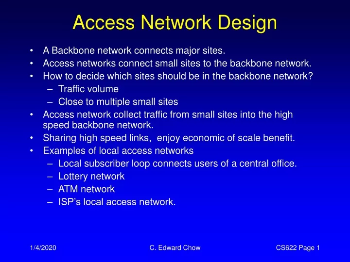
Access Network Design • A Backbone network connects major sites. • Access networks connect small sites to the backbone network. • How to decide which sites should be in the backbone network? • Traffic volume • Close to multiple small sites • Access network collect traffic from small sites into the high speed backbone network. • Sharing high speed links, enjoy economic of scale benefit. • Examples of local access networks • Local subscriber loop connects users of a central office. • Lottery network • ATM network • ISP’s local access network. C. Edward Chow
A Simple Access Design • 7 nodes. N1 is the backbone site. Symmetric traffic. Piecewise linear cost: Fixed cost=400$3.00/km/mofirst 300km $1.75/km/moafter 300km C. Edward Chow
Star • Cost=$9650; Max. Utilization=23.2% C. Edward Chow
Cheaper Local-Access Design • N2 serves as a concentrator for N6 and N7. • Local link can use shorter less expensive link. C. Edward Chow
Two concentrators • N2 for N6 and N7; N4 for N3. C. Edward Chow
Move to MST • Choose N7 as concentrator instead of N2. Become MST C. Edward Chow
MSTs not always Optimal Access Designs • When traffic grows 50%, MST costs $10,616 and the links to concentrators N4 and N7 must have two links to keep utilization below 50%. C. Edward Chow
An Optimal Design • Constraint MST problem. Note that N3 connect directly to N1 since through N4 will violate the utilization constraint. C. Edward Chow
Frame Relay Design • Current frame relay provide permanent virtual circuit (PVC). They are moving to offer Switched virtual circuit (SVC). • PVC is fixed pipe. SVC is dialed pipe. • Packets exceed Committed Information Rate (CIR) will have discard eligibility (DE) bit set. • Three classes of charges: access link costs, provider port costs (cost to frame relay), and CIR costs. • It is volume dependent and not distance dependent. Port Charges CIR charges per PVC C. Edward Chow
Frame Relay vs. Lease-Line Cost • Let x be the distance from the site to the center. • Fixed cost=$400/month; $3.00/km/month. • Leased-line cost=6*400+6*3.00*x • Assume frame relay provider has point of presence (pop) at each site. Each site connects to the frame relay network. • N1 uses 128 kbps link, others use 56kbps links. • Port charges=6*250+500=2000. • Access charges=7*(400+3.0*20)=7*460=3220 • CIR charges=4*30+2*25=170 if 4 PVCs with 16kbps CIR and 2PVCs with 8kbps. • Frame relay cost=2000+3220+170=$6290/mo • Solve 2400+18*x=6290 x=216.11 km. Break even point. • Most WAN are larger than this Frame Relay is a good candidate. C. Edward Chow
Choosing Backbone Nodes • Definition 5.1: Given a set of sites Ni and traffic matrix T(i,j), weight(Ni)=Sj(T(i,j)+T(j,i)). • Sometimes, the weights of nodes indicate the choices of backbone nodes or traffic centers. • Design Principle 5.3: It is acceptable for small nodes to route their traffic via big nodes, but generally we do not want to route the traffic between big nodes via the small nodes. C. Edward Chow
3 Types of Local Access Problems • Access node’s traffic are considerably smaller than the smallest link. But occasionally, they may need to download huge file Use frame relay or access tree (capacitated spanning tree building problem.) • Access node’s traffic is comparable to the capacity of the smallest link. Choices: connect them directly to hub or put concentrator between hub and those nodes. (Concentrator placement problem, local access tree problem.) • Access node’s traffic can fill several low-speed access lines. Choices: multiple links to multiple backbone nodes; or high speed link to a backbone node. They are nature choices for concentrator locations. C. Edward Chow
One-speed One-Center Design • Example: 19 nodes to a hub, N14. • 4 sites can share a line. Each link is 1200 bps. • Use 9600 bps link. 50% utilization. • The problem becomes a tree building problem. • Solution: • SPT • MST • Prim-Dijkstra with 0<a<1. • Other algorithm? C. Edward Chow
SPT(Star) • Cost=$26358 C. Edward Chow
MST • $18,730 C. Edward Chow
Prim-Dijkstra with a=0.3 • $15930. N11 can go through N4; Two clusters with N18 and N9 as concentrators. C. Edward Chow
How Many possible Trees to Search for Optimal Designs? • Cayley’s Theorem: Given n nodes, there are nn-2 different spanning tree. • For 20 nodes, there are 2018=2.621*1023 trees. C. Edward Chow
Constraint Minimum Spanning Tree Problem • It solves the problem of creating capacitated (constraint) minimum spanning tree (CMST). • CMST problem: Given a central node N0 and a set of other nodes (N1, …, Nn), a set of weights(w1,…,wn) for each node, the capacity of a link, W, and a cost matrix Cost(I,j), find a set of trees T1, …, Tk such that each Ni belongs to exactly one Tj and each Tj contains N0, and C. Edward Chow
Greedy CMST Algorithm Sort the edges according to the cost. s1: Take the lowest cost edge from sorted list.Add it to the solution subtrees if the addition does not violated the constraingo to s1. Assume W=3, each node has wi=1, and the following topology: C. Edward Chow
Esau-William Algorithm • Initially, each node starts off in a tree with itself. • Compute the tradeoff function:Tradeoff(i,j)=minj Cost(i, j)-Cost(Comp(ii),Center)where Cost(Comp(i),Center) is the cost of connecting the component with Node i to the center. It is equivalent to the cost of the shortest path from the Center to any node in the component. Cost(i,j) is the link cost from Node i to Node j. minj Cost(Ni,Nj) suggests pick the closest neighboring Node j. • Maintain a sorted list of links based on the Tradeoff() value. • Actually, in each iteration, we only consider the shortest link out of a node to a neighbor that does not belong the component of the node. • L1: adds the top link in the list to the solution if the weight constraint of the component is satisfied. otherwise reject it. • update the tradeoffs in other links due to the newly added link and resort the list. • got to L1. C. Edward Chow
Apply Esau-William Algorithm • Assume W=3, each node has wi=1, and the following topology: • Tradeoff(1,3)=minj Cost(1,J)-Cost(Comp(1),Center)=minj Cost(1,3)-7 //comp(1) contains N1=5-7=-2 // pick closest neighbor, Node 3 • Tradeoff(2,0)=6-8=-2 • Tradeoff(3,1)=5-11= -6 • Tradeoff(4,2)=7-14= -7 • Tradeoff(5,3)=8-17= -9 • Tradeoff(5,3) is lowest one. • Accept link(5,3) to the solutionsince weight constraint on component with nodes 5 and 3 are not violated.SWi=W5+W3=2<=W=3 • Effectively this picks the faraway nodewith short link to its neighbor and group them as component. C. Edward Chow
Apply Esau-William Algorithm(2) • Update Tradeoff(5,4)=9-11= -2Next shortest link out of 5 is (5,4)(Comp(5)=11,node 5 goes through node 3 to center)Tradeoff(3,1)=5-11= -6 not changed. • Tradeoff(1,3)=5-7= -2 • Tradeoff(2,4)=6-8= -2 • Tradeoff(4,2)=7-14= -7 • Tradeoff(5,4)=9-11= -2 • Pick Tradeoff(4,2) lowest • Accept link(4,2) sinceweight constraint on component with nodes 4 and 2 are not violated.SWi=W4+W2=2<=W=3 C. Edward Chow
Apply Esau-William Algorithm(3) • Update Tradeoff(4,3)=8-8= 0Tradeoff(2,1)= -2 not changed. • Tradeoff(3,1)=5-11= -6 • Tradeoff(5,4)=9-11= -2 • Tradeoff(1,3)=5-7= -2 • Tradeoff(2,1)=6-8= -2 • Tradeoff(4,3)=8-8= 0 • Pick Tradeoff(3,1) • Accept link (3,1) sinceweight constraint on component with nodes 1, 3 and 5 are not violated.SWi=W1+W3 +W5 =3<=W=3 • Since nodes 5 and 3 now go through node 1 to Center,update Tradeoff(5,4)=9-7=2Tradeoff(3,4)=8-7= 1Tradeoff(1,2)=6-7= -1 C. Edward Chow
Apply Esau-William Algorithm(4) • Tradeoff(5,4)=9-7=2 • Tradeoff(3,4)=8-7=1 • Tradeoff(1,2)=6-7= -1 • Tradeoff(2,1)=6-8= -2 • Tradeoff(4,3)=8-8=0 • Tradeoff(2,1) is lowest butadd link(2,1) result a componentwith 5 nodes violate Swi<=3. • Reject(2,1) recompute Tradeoff(2,0)=8-8=0 • Reject(1,2) similar reason. Recompute Tradeoff(1,0)=7-7=0 • Pick link(1,0) • Pick link(2,0) complete the access network. C. Edward Chow
Creditability of Esau-Williams Algorithm • 1-exchange test: no cheaper link can be substituted for an existing link without violating the capacity constraints. For homogeneous traffic, 4 sites on a line Considerpretty good! C. Edward Chow
Esau-Williams and InHomogenous Traffic C. Edward Chow
Line Crossing and Esau-Williams C. Edward Chow
Sharma’s Algorithm • Compute the angle s from each site S to the central site C. If S and C have the same coordinate, set s =0. • Sort the angles s . • Beginning at a site Sfirst, create a set of nodes clockwise (or counterclockwise) from Sfirst.A set is complete when adding the next node would put Ssetw(site) > W. The next set starts with that node. • The design is completed by building a MST on each set with the addition of the central node C. Note that the CMSTs do not have line crossing. Each has edges within some range from the central site. C. Edward Chow
Sharma’s Algorithm Result C. Edward Chow
Creditability of Sharma Algorithm • Much higher failure rate than Esau-Williams’. C. Edward Chow
Sharma vs. Esau-Williams EW_Ratio=SharmaCost/EWCost; S_Ratio=1/EW_Ratio C. Edward Chow
Multispeed CMST Problem • Find the tree rooted at N0, s.t.And is minimum. • Here pred(N) is a predecessor function that leads towards the root. • Ancestor of N are nodes, N’, such that predn(N’)=N for some n > 0. • C(i,j,k) is the cost matrix which give the cost of a link of type Lk between Ni and Nj. C. Edward Chow
Multispeed Local Access Algorithm (MSLA) • Assign each node the smallest link l possible to connect it to the center. Compute spare_capacity(n)=Wl-wn. • Create trade-off heap for n similar to Esau-Williams.The trade-offs represent the saving from linking site n to site rather than directly link to the center.Allow upgrade links to carry additional traffic.Tradeoffn(I)=c(n,i, l)+Upgrade(i,wn)-c(n,0,l) Upgrade(i,wn ) is the cost of adding wn units to the links that connect i and 0. • Add the edges as long as the tradeoffs are less than or equal to zero. Terminate when tree is built. C. Edward Chow
MSLA Example spare_capacity(1)=0.5*56000-20000=8000 spare_capacity(2)=0.5*9600-2400=2400 spare_capacity(3)=0.5*56000-9600=18400 spare_capacity(4)=0.5*9600-4800=0 • Initial State (Utilization=0.5) 012 C. Edward Chow
MSLA (2) • N2 is furthest away from N0. It is closer to N4. • For N2 to go through N4, require (4,0) to upgrade from 9600 to 56000. It is c(4,0,1) – c(4,0,0). • Tradeoff2(4)=c(2,4,0)+(c(4,0,1)-c(4,0,0))-c(2,0,0).Not pick. • N4 goes through N3, no upgrade is needed. It is the best tradeoff. • Next, the most attractive tradeoff is route N2 through N3. Again no upgrade is needed. • Finally, connect N3 to N1 and increase (1,0) to 128kbps link. C. Edward Chow
MSLA (3) C. Edward Chow
Esau Williams20 nodes with 9.6kbps links C. Edward Chow
MSLA 20 nodes with multispeed links C. Edward Chow
MultiCenter Local-Access (MCLA) Problem Given • a set of backbone sites B=(B0,…,Bm) • a set of access nodes N=(N1,…,Nn) • A set of weights (w1,…,wn) for each access node, • A cost matrix Cost(i,j) for each backbone/access pair Find a set of trees T1,…,Tk s.t. • Exactly 1 backbone site belongs to each tree • SNiTjwi<W • STreesSlLinks Cost(endll,end2l) is minimum. C. Edward Chow
Nearest-Neighbor Esau-Williams Algorithm NNEW: • For each b in B, let Sb={ nN | Cost(n,b) < Cost(n,b’) b’B}If n is equidistant between several backbone nodes, add n to one Sb at random. • Use Esau-Williams to construct a capacitated MST on each set bSb. • Example:circlebackbone nodesquareaccess node • A definite belong to X • B, C, and D not clear. C. Edward Chow
Creditability Test • Test Exchange leave node to a different tree and see if it reduces the cost. NNEW creditability not good C. Edward Chow
MultiCenter Esau-Williams • MCEW algorithm (Kershenbaum-Chou): Replace the tradeoff function as Tradeoff(i,j)=minj Cost(i, j)-Cost(Comp(i),Center(i)) • Initially, we set Center(i) to be the closet center. • As node i is merged with node j, update Center(i)=Center(j). C. Edward Chow
NNEW vs. MCEW • Slight cost advantage of using MCEW. • MCEW is more creditable. C. Edward Chow
Practical Considerations • Some access trees contain too many nodes.Solution: add additional test/constraints that prohibit the merge of two components with too many nodes. • Some access trees contain too many hops.Solution: add depth checking constraint. • Some site in the access tree has too many links.Solution: add degree constraint. • A central site has too many links.Solution1: Modify the tradeoff function as Tradeoff(i,j)=minj Cost(i, j)-a*Cost(Comp(i),Center))where a > 1. By adjust a we limit the links connect to a center.Solution 2: Use NNEW or MCEW with initial center assignment of some nodes to low utilization center. • Some site fails too often.Solution: Mark it as not being choice for predecessor of other sites. C. Edward Chow
Homework #6: Local Access Design Given the topology below, the weight of each node is 1, and W = 3 a) apply the greedy CMST algorithm. b) apply the Esau-Williams algorithm. Highlight the trees (components) selected. C. Edward Chow
Solution to Hw#6 Solution a): Greedy MST. First sort the edge cost in increasing order. C. Edward Chow
Solution to Hw#6(2) Solution b) Esau-Williams Algorithm begin by computing the tradeoffs for the nearest neighbors of each node (since that link will have smallest cost and yield a low trade-off values): t14 = c14 - cc1 = 1 - 2 = -1 t23 = 1 - 8 = -7 t32 = 1 - 11 = -10 t41 = 1 - 14 = -13 t53 = c53 - cc5 = 2 - 5 = -3 starting with t41 which is the lowest tradeoff value, we add link (4,1) to subtrees,now cc4 = 2 since node 4 now connected to the center through node 1, find the next nearest neighbor of 1 to be 0, t10=2-2=0let us now compute the tradeoff between node 4 and the next nearest neighbor to node 4 (which is node 2), t42 = c42 - cc4 = 5 -2 = 3 C. Edward Chow
Solution to Hw#6(3) Now t32 has the lowest tradeoff value, add link (3,2) to the subtrees,now cc3 = 8 and the next nearest neighbor to node 3 is 5, t35 = 2 - 8 = -6 We also need to update t23 since (2,3) is chosen. The next nearest neighbor to node 2 is 4, t24 = 5 - 8 = -3 Select t35=-6, add link(3,5) to the subtrees. N ow Cc2=Cc3=Cc5=5, we need to update t31=7-5=2 t24=5-5=0 t50=5-5=0 Select (1,0) add link (1,0) to the subtrees. Reject (2,4) since it will create a component of weight = 4. Select (5,0) add link (5,0) to the subtrees. Now all nodes are connected to node 0. Note that the algorithm always terminates with links whose tradeoffs are 0. We will never consider any links with positive tradeoff. C. Edward Chow
Solution to Hw#6(4) The solution has a cost of 11. Both EW algorithm and GMST find optimal solution but GMST is much faster. C. Edward Chow