Overview of Inner Silicon Detector Alignment in RHIC/STAR Experiment

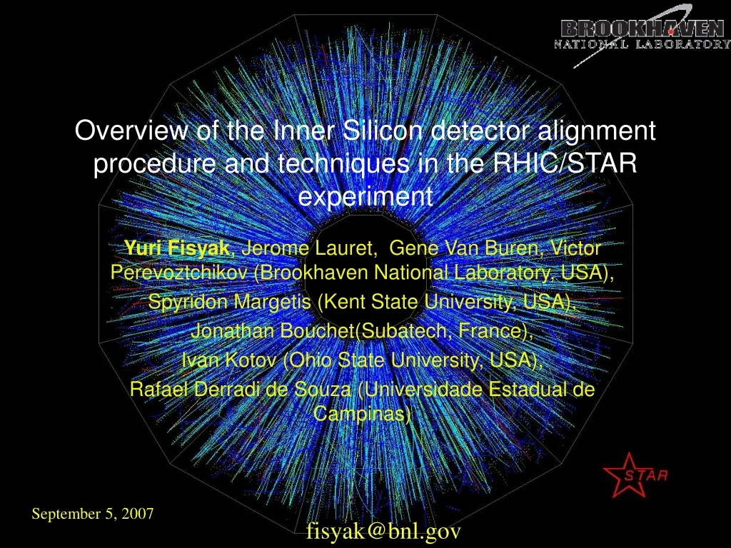
1. Overview of the Inner Silicon detector alignment procedure and techniques in the RHIC/STAR experiment Yuri Fisyak, Jerome Lauret, Gene Van Buren, Victor Perevoztchikov (Brookhaven National Laboratory, USA), Spyridon Margetis (Kent State University, USA), Jonathan Bouchet(Subatech, France), Ivan Kotov (Ohio State University, USA), Rafael Derradi de Souza (Universidade Estadual de Campinas) September 5, 2007 fisyak@bnl.gov

2. Outline • STAR detector. • STAR tracking in barrel region : TPC + SVT + SSD. • Results of two drift detectors SVT and TPC alignment with respect to each other for run III and IV data. • Reiteration with alignment procedure for run V (Cu+Cu 200 GeV) data and our plans for run VII (Au+Au 200 GeV): • Impact of SSD on alignment, • Interest in charm, • Limitations from Detector setup due to Multiple Coulomb Scattering, • Requirements on Silicon detectors alignment precision. • Methods, Calibration and Alignment procedure. • Results. • Conclusion.

3. RHIC

4. STAR - Solenoidal Tracker At RHIC - A multi-purpose detector for Heavy Ions Physics

5. Time Projection Chamber (TPC) FTPCs (1 +1) Vertex Position Detectors The STAR Detector Magnet Coils Silicon Vertex Tracker(SVT) Silicon Strip Detector (SSD) Central Membrane ZCal ZCal Endcap Calorimeter BZ= 5kG Barrel EM Calorimeter Central Trigger Barrel + TOF patch

6. Time Projection Chamber • TPC is the main STAR tracking detector [1] and working in STAR from day one (Run I, FY 2000). • TPC is divided into halves by Central Membrane and contains 12 sectors in each half and each sector contains Inner (13 pad rows) and Outer (32 pad rows) sub sectors. • Electrons produced by charge particles drift (in Z direction) from Central Membrane to end caps in almost parallel electric and magnetic fields where they are detected with 45 pad rows placed at radii in range [60,190] cm. • Drift velocity is monitored by laser system[2] with precision ~2 10-4 providing systematic error in Z direction ~40 m at the maximum drift length (~ 2m). • Spatial resolutions: • ≈ 600 m and z ≈ 1200m for Inner Sectors and •  ≈1200 m and z ≈ 1600m for Outer Sectors. • Distortions due to non-perfect electric field and space charge collected in TPC are monitored by DCA (distance of closest approach) of the track at the primary vertex and kept on the level better than ~100µm[3].

7. SVT is the inner tracking-detector in STAR and it is located near the interaction point. Two hybrids form a wafer, and wafers form a ladder, ladders are arranged in 3 barrels on two rigid Clam-Shells. The detector consists of 216 wafers in total. SVT- A 3 Layer Silicon Drift Detector[4]. • A new technology at the time. • Primarily designed to do multi-strange particle physics. • Electrons drift in  direction (perpendicular to TPC drift direction). • Strips (=anodes) are placed along Z (beam axis). • Size of pixel   Z = 250 m (time bin)  250 m (strip pitch). • The intrinsic spatial resolution (accounting for charge sharing): •  < 80m and • z < 80m. • Relatively thick (~1.5% X0 per layer). • Relatively far from beam. • Installed in STAR since Run II, and became fully functional since Run III. Barrel 1: • 8 ladders; • 4 wafers each ladder; • <R> = 6.85 cm. Barrel 2: • 12 ladders; • 6 wafers each ladder; • <R> = 10.8 cm Barrel 3: • 16 ladders; • 7 wafers each ladder; • <R> = 14.7 cm.

8. It wraps around the SVT as a fourth layer. • Its primary purpose is to provide an intermediate (non-drifting) point for track matching between TPC and SVT. • 20 ladders with 16 wafers each mounted on 4 rigid Sectors at ~23 cm from the beam. • Installed in STAR for Run IV, became fully functional in Run V. • Strip pitch: 95 m. Strip length: 4 cm. Stereo angle between p- and n-strips is 35 mrad. • Intrinsic resolution should be better than ~30 m ()  860 m (Z). • BigAdvantage: Non-drifting technology. • Of course there is a Lorentz shift of holes and electrons in  direction due to our 5 kG magnetic field (with Lorentz holes = 4.4°  4.4m and electrons = 1.6 °  1.6 m) which produces a sizable effect in Z direction ( ~ 200m) due to the stereo angle. But it is clear how to account for this effect. SSD - A single layer of 2-side Silicon Strip Detector[5] ~70 cm

9. Alignment and Calibration of SVT with TPC for Run III-IV data • Analysis of the first SVT data with respect to TPC • has showed rather weak correlation between the data and SVT calibration and alignment done on test bench and • clearly required recalibration and realignment in situ. • These recalibration and alignment efforts for these two drifting detectors gave rather modest results: spatial resolution (including alignment)  ≈ Z ≈ 200 µm. • However these modest results could not be used in heavy ion collision high track multiplicity environment due to a high ghosting level. • We had to revisit this problem when the SSD came into the game.

10. New goals • The initial goal for the SVT was to measure particles, but this task pretty much has been done with TPC only analysis. • But there is much interest in direct charm measurements now. • In Cu+Cu 200 GeV interactions (Run V) we have already observed ~4 standard deviations of D0 signal. • Thus it looks very attractive to set a worthy task to reducebackground and enhance significance of the charm signal by a factor of ~3-5 through use of the Silicon Vertex Detector. • A renewed effort started with SSD coming online. • Alignment and drift velocity calibrations were re-visited to see if we are able to do ‘some/any’ direct D-meson measurement and/or B-meson tagging. • I have to stress: • Heavy Ion collisions are the toughest environment for this kind of work: about 2000 tracks in a single event !

11. Figures of merit for SVT/SSD precision. • Pointing accuracy, aka Impact parameter resolution: • DCA resolution (in bending XY  plane: DCA) and • Resolution in non-bending plane: z, is figure of merit for charm decay (c~100mm) registration with a vertex detector: • 2DCA= 2vertex+ 2track + 2MCS (the same for non-bending plane), • primary vertex resolution: vertex ~ 600 mm / √Ngood tracks, for central Au+Au collisions turns out to be better than 20 mm (for minimum biased events ~100 mm), • track pointing resolution: track ~ 2 XY in our case, where XY is intrinsic detector precision  alignment errors, • Multiple Coulomb Scattering (MCS): MCS ~ 170mm / p(GeV/c) (from simple analytic estimations) • from requirement that the track pointing resolution should be comparable with MCS @ 1 GeV/c then detector resolution (including alignment) should be XY < 80 mm and z < 80 mm for both bending and non-bending planes.

12. Methods • Methods can naturally be split into two parts: • Calibration of SVT Drift velocities on hybrid level, and • Alignment of detectors: • Assumed: • Frozen wafer position on ladder from survey data, i.e. ladder is the lowest level degree of freedom. • Rigid body model: ignore possible twist effects, gravitational/stress sagging etc. • The methods are interconnected and this supposes iterative procedure i.e. • using average drift velocities to do alignment and • after the alignment, check and correct drift velocities • …and iterate

13. Methods (average drift velocities) • As the first approximation we are using average (constant) drift velocityper hybrid from charge step method: • clean up noisy strips, • from drift time distribution for each hybrid we have reasonably sharp cut offs at t0 and tmax, • from these numbers and the total drift length (L) we can estimate average drift velocity vD = L/(tmax - t0). • These hybrids’ vD shouldbe correct in averageper ladder; this is the sample which we are using for alignment. t0 tmax Drift Time (time bins)

14. Methods (alignment) I • For small misalignments, we can assume a model where the hit position deviations from tracks are linearly proportional to the misalignments through derivatives of track projections to measurement planes with respect to misalignment parameters (e.g. first order of a Taylor expansion) • The derivatives take as a condition that both a track prediction and a hit stay on a measurement plane after applying the correction (see Appendix for details) • Global alignment: • Vector of misalignment parameters:  (shift+rotation = 6 parameters) • Coordinates: X = (x,y,z) • Xhit - X = ∂X/ ∂ G, whereXhitand X are hit position and track prediction on measurement plane, respectively • Local alignment: • Vector of misalignment parameters:  • Coordinates: u = (u,v,w0) • uhit - u = ∂u/∂ L, where u is prediction of track on measurement plane [6].

15. Methods (alignment) II • Misalignment parameters have been calculated as slopes of straight line fits to histograms of the most probable deviations (Xhit - X or uhit - u) versus the corresponding derivative matrix (Gij or Lij) component [7] • See examples on following slides • For alignment we use “good” (with well defined parameters) tracks fitted with the primary vertex. • Use of primary tracks significantly improves precision of track predictions in Silicon detectors and reduces influence of systematics. • Precision of the method is checked with simulation • Accuracy ~10 m in detector position and ~0.1 mrad in its rotation. • There is a problem when we start far from minimum because there are significant correlations among alignment parameters. • To solve this problem as a starting point we use Least-Squares Fitwith above derivatives to get first approximation for the parameters. • The precision of this method is less than slopes method but it does provide a reasonable approximation to use slopes.

16. An example of Global alignment of the first SSD sector: is rotation around Z axis deviations of hit position from track prediction slope Derivatives

17. An other example of local alignment:  is rotation around w (local Z) axis • hit position deviations • Derivative • slope

18. Example of correcting a SSD individual ladder rotation around the v-axis (local Y) (). AFTER BEFORE  = 16.36 ± 0.40 mrad  = 0.31 ± 0.45 mrad

19. Procedure includes 4 steps: • Average SVT drift velocity: as the first approximation, average drift velocity for SVT is obtained from charge step method for each hybrid. • TPC only tracks • Global alignment of SSD with respect to TPC as whole • Global alignment of SSD sectors • Local Alignment of SSD ladders: • Individual Ladders showed translations up to ~200 m and rotations (especially around y-axis) of up to ~20mrad. • After the SSD Ladder fine tuning, the majority of ladders had translational alignments calibrated to under 20m, and rotational alignment calibrated to within 0.5 mrad, both of which were within errors of the calibration method. • TPC + SSD tracks • Global Alignment of SVT as whole • Global Alignment of SVT Clam Shells • Local Alignment of SVT ladders • Correction to SVT drift velocities. • SVT drift velocities have been refitted including extra dependence on drift distance and anode (up to 3rd degree Tchebyshev, see next slide). This fit reduced hit residuals from ~100 m to ~10 m. • TPC + SSD + SVT tracks • Check consistency • Reevaluate SVT & SSD hit errors

20. An example of drift residual (cm) versus drift distance before and after the correction (typical wafers) Before After Down to ~10 µm in means Before After ± (Drift Distance / max Drift Distance + 0.1) for left / right hybrid

21. SVT/SSD resolutions after Calibration/Alignment • A quality of calibration/alignment procedure for Run V has been estimated from hit pull analysis in track fit, and • Spatial resolution estimated by requirement to have pull standard deviation equal to 1 (averaged over 3 samples: 62 GeV Forward Magnetic Field, 200 GeV Reverse and Forward Magnetic Field) is as follows: • SVT: • = 49±5 m, and • Z = 30±7 m. • SSD resolution: •  = 30 m (set to design value since << MCS), • Z = 742 ± 41 m.

22. Pointing (DCA) resolution has been estimated as standard deviation of global track DCA with respect to the primary vertex. • With increasing no. of fitted Si points it is improved by ~ order of magnitude. • Contribution from tracking (constant term) is comparable with MCS @ 1 GeV/c • Thus we have reached our desired goal ! DCA resolution XY Z

23. The SVT enhances physics signals.(Ξ- Analysis Comparing TPC Only and TPC+SVT production for Cu+Cu 62 GeV, analysis done by Geraldo Magela S. Vasconcelos, UNICAMP -Brazil) TPC only TPC+SVT We get 20% enhancement of  signal. Zvert<30cm

24. Conclusions • Recent interest in charm physics has re-focused STAR’s interest in its vertex detectors. • The presence of drift silicon (SVT) technology complicates the alignment task • but also presence of non-drifting detectors (like SSD) improve the situation drastically. • Our alignment approach and techniques were successful to overall shifts better than 20 m • which is sufficient for this device. • Calibration/alignment procedure for Run V (Cu+Cu) has been completed, data has been re-processed, and data analyses is under way. • Calibration/alignment procedure for Run VII (Au+Au 200 GeV) is under way. • First physics checks (Run V) look fine. Silicon detectors: • improve momentum resolution for global tracks, • improve primary vertex resolution, • greatly improve track selection (based on DCA), • sharpen (multi-)strangeness physics, and • other non-physics side benefits: • Use of SVT (+SSD) as a high resolution microscope to undo TPC distortions and as a distortion monitor in high luminosity runs. • STAR Silicon Vertex Detector (and Silicon Strip Detector) are sharpening our physics.

25. References • “The STAR time projection chamber a unique tool for studying high multiplicity events at RHIC”, M.Anderson et al., NIM A499: 652,2003. • “The laser system for the STAR time projection chamber”, J. Abele et al., NIM A499: 692,2003. • “Correcting for distortions due to ionization in the STAR TPC”,
G. Van Buren et al.,NIM A566:22-25,2006. • “The STAR Silicon Vertex Tracker” A large area Silicon Drift Detector”, R.Bellwied et Al., NIM A499: 640, 2003. • “The STAR silicon strip-detector (SSD)”, L.Arnold et al., NIM 2003 A499: 652, 2003. • “Alignment Strategy for the SMT Barrel Detectors”, D.Chakborty, J.D.Hobbs, October 13, 1999. D0 Note (unpublished) • “Sensor Alignment by Tracks”, V.Karimaki et al.,CMS CR-2004/009 (presented at CHEP 2003)

26. Appendix