Download
1 / 26
270 likes | 407 Views
Learning Classifiers For Non-IID Data. Balaji Krishnapuram , Computer-Aided Diagnosis and Therapy Siemens Medical Solutions, Inc. Collaborators: Volkan Vural, Jennifer Dy [North Eastern], Ya Xue [Duke], Murat Dundar, Glenn Fung, Bharat Rao [Siemens] Jun 27, 2006. Outline.

E N D
Learning Classifiers For Non-IID Data Balaji Krishnapuram, Computer-Aided Diagnosis and Therapy Siemens Medical Solutions, Inc. Collaborators: Volkan Vural, Jennifer Dy [North Eastern], Ya Xue [Duke], Murat Dundar, Glenn Fung, Bharat Rao [Siemens] Jun 27, 2006
Outline • Implicit IID assumption in traditional classifier design • Often, not valid in real life. Motivating CAD problems • Convex algorithms for Multiple Instance Learning (MIL) • Bayesian algorithms for Batch-wise classification • Faster, approximate algorithms via mathematical programming • Summary / Conclusions
IID assumption in classifier design • Training data D={(xi,yi)i=1N: xi2 Rd, yi2 {+1,-1}}, • Testing data T ={(xi,yi)i=1M: xi2 Rd, yi2 {+1,-1}}, • Assume each training/testing sample drawn independently from identical distribution: (xi,yi) ~ PXY(x,y) • This is why we can classify one test sample at a time, ignoring the features of the other test samples • Eg. Logistic Regression: P(yi=1|xi,w)=1/(1+exp(-wT xi))
Evaluating classifiers: learning-theory • Binomial test set bounds: With high probability over the random draw of M samples in testing set T, • if M large and a classifier w is observed to be accurate on T, • with high probability its expected accuracy over a random draw of a sample from PXY(x,y) will be high • If the IID assumption fails, all bets are off ! • Thought experiment: repeat same test sample M times
Training classifiers: learning theory • With high probability over the random draw of N samples in training set D, the expected accuracy on a random sample from PXY(x,y) for the learnt classifier w will be high iff • accurate on the training set D; and N large • satisfies intuition before seeing data (“prior”, large margin etc) • PAC-Bayes, VC-theory etc rely on iid assumption • Relaxation to exchangeability being explored
Additive Random Effect Models • The classification is treated as iid, but only if given both • Fixed effects (unique to sample) • Random effects (shared among samples) • Simple additive model to explain the correlations • P(yi|xi,w,ri,v)=1/(1+exp(-wT xi–vT ri)) • P(yi|xi,w,ri)=s P(yi|xi,w,ri,v) p(v|D) dv • Sharing vT ri among many samples correlated prediction • …But only small improvements in real-life applications
Candidate Specific Random Effects Model: Polyps Sensitivity Specificity
CAD algorithms: domain-specific issues • Multiple (correlated) views: one detection is sufficient • Systemic treatment of diseases: e.g. detecting one PE sufficient • Modeling the data acquisition mechanism • Errors in guessing class labels for training set.
The Multiple Instance Learning Problem • A bag is a collection of many instances (samples) • The class label is provided for bags, not instances • Positive bag has at least one +ve instance in it • Examples of “bag” definition for CAD applications: • Bag=samples from multiple views, for the same region • Bag=all candidates referring to same underlying structure • Bag=all candidates from a patient
CH-MIL Algorithm for Fisher’s Discriminant • Easy implementation via Alternating Optimization • Scales well to very large datasets • Convex problem with unique optima
Lung CAD *Pending FDA Approval AX Computed Tomography Lung Nodules& Pulmonary Emboli DR CAD
Classifying a Correlated Batch of Samples • Let classification of individual samples xi be based on ui • Eg. Linear ui = wT xi ; or kernel-predictor ui= j=1Nj k(xi,xj) • Instead of basing the classification on ui, we will base it on an unobserved (latent) random variable zi • Prior: Even before observing any features xi (thus before ui), zi are known to be correlated a-priori, • p(z)=N(z|0,) • Eg. due to spatial adjacency = exp(-D), • Matrix D=pair-wise dist. between samples
Classifying a Correlated Batch of Samples • Prior: Even before observing any features xi (thus before ui), zi are known to be correlated a-priori, • p(z)=N(z|0,) • Likelihood: Let us claim that ui is really a noisy observation of a random variable zi : • p(ui|zi)=N(ui|zi, 2) • Posterior: remains correlated, even after observing the features xi • P(z|u)=N(z|(-12+I)-1u, (-1+2I)-1) • Intuition: E[zi]=j=1N Aij uj ; A=(-12+I)-1
SVM-like Approximate Algorithm • Intuition: classify using E[zi]=j=1N Aij uj ; A=(-12+I)-1 • What if we used A=( + I) instead? • Reduces computation by avoiding inversion. • Not principled, but a heuristic for speed. • Yields an SVM-like mathematical programming algorithm:
Conclusions • IID assumption is universal in ML • Often violated in real life, but ignored • Explicit modeling can substantially improve accuracy • Described 3 models in this talk, utilizing varying levels of information • Additive Random Effects Models: weak correlation information • Multiple Instance Learning: stronger correlations enforced • Batch-wise classification models: explicit information • Statistically significant improvement in accuracy • Only starting to scratch the surface, lots to improve!