Download
1 / 21
210 likes | 605 Views
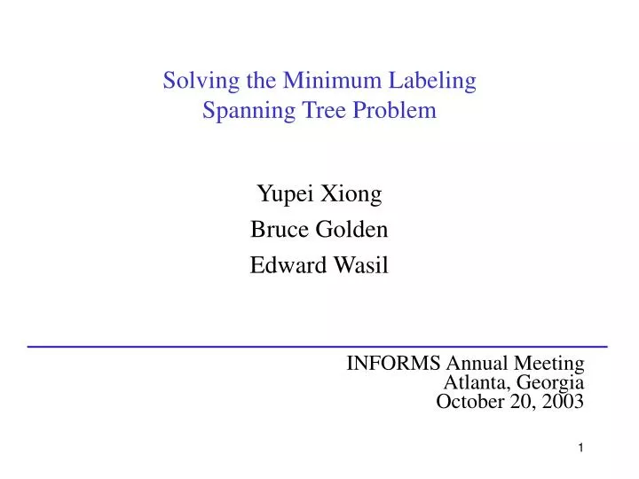
Solving the Minimum Labeling Spanning Tree Problem Yupei Xiong Bruce Golden Edward Wasil INFORMS Annual Meeting Atlanta, Georgia October 20, 2003 Introduction The Minimum Labeling Spanning Tree (MLST) Problem Communications network design

E N D
Solving the Minimum LabelingSpanning Tree Problem Yupei Xiong Bruce Golden Edward Wasil INFORMS Annual Meeting Atlanta, Georgia October 20, 2003
Introduction • The Minimum Labeling Spanning Tree (MLST) Problem • Communications network design • Edges may be of different types or media (e.g., fiber optics, cable, microwave, telephone lines, etc.) • Each edge type is denoted by a unique letter or color • Construct a spanning tree that minimizes the number of colors
3 2 5 3 4 2 5 4 6 1 e c e d 6 1 a e e a d b b b b b b Introduction • A Small Example InputSolution
Literature Review • Where did we start? • The MLST Problem is NP-hard • Several heuristics had been proposed • One of these, MVCA (version 2), was very fast and effective • Worst-case bounds for MVCA (versions 1 & 2) had been obtained
Literature Review • An optimal algorithm (using backtrack search) had been proposed • On small problems, MVCA (version 2) consistently obtained nearly optimal solutions • See [Chang & Leu, 1997], [Krumke & Wirth, 1998], and [Wan, Chen & Xu, 2002]
A Perverse-Case Example for MVCA (version 2) • MVCA (version 2) • It might add colors associated with 3 polygons first • Then, it must add colors associated with 4 rays • Optimal Solution • Add colors associated with 4 rays first • Then, add color associated with 1 polygon Input e d c e d b e d a c a b b a c a g f b f g c f g
A Perverse Family of Graphs for MVCA (version 2) • Given an integer k 3, build a graph G = (V, E) with k2 nodes and 2k – 1 labels, where the edges form k –1 concentric polygons and k rays (as below for k = 3) e e b b a a a d c d c b • In the previous example (on page 6), we had k = 4 and
A Remedy for MVCA (version 2) • In general, the result , which approaches 2 for large k, is possible • We present a remedy which leads to MVCA (version 3) • MVCA (version 3) finds the optimal solution for each perverse-case example • In computational experiments, MVCA (version 3) consistently outperforms MVCA (version 2) by a small amount • Running times are essentially the same
MVCA (version 3) • Definition: A label c is called a cut label if the removal of all edges with label c disconnects graph G • Description of MVCA (version 3) a. Add all cut labels to obtain C, the set of used labels b. Let H be the subgraph of G restricted to edges with labels from C c. If H is connected and spans all nodes in V, go to f
MVCA (version 3) d. Repeat d1. Let H be the subgraph of G restricted to edges with labels from C d2. For all , determine the number of components when adding all edges with label i to H d3. End For d4. Choose label i with the smallest resulting number of components: C C {i} e. Until H is connected and spans all nodes in V f. Find an arbitrary spanning tree of H
Some Observations • The labels associated with the rays in the perverse-case example are cut labels • These labels must be in any solution • MVCA (version 3) adds these labels first • Unlike the MST, where we focus on the edges, here it makes sense to focus on the labels or colors • Next, we present a genetic algorithm (GA) for the MLST problem
Genetic Algorithm: Overview • Randomly choose p solutions to serve as the initial population • Suppose s [0], s [1], … , s [p – 1] are the individuals (solutions) in generation 0 • Build generation k from generation k – 1 as below For each j between 0 and p – 1, do: t [ j ] = crossover { s [ j ], s [ (j + k) mod p ] } t [ j ] = mutation { t [ j ] } s [ j ] = the better solution of s [ j ] and t [ j ] End For • Run until generation p – 1 and output the best solution from the final generation
Crossover Schematic (p = 4) S[2] S[3] Generation 0 S[1] S[0] S[2] S[1] S[3] S[0] Generation 1 S[2] S[1] S[0] S[3] Generation 2 S[1] S[2] S[3] S[0] Generation 3
Crossover • Given two solutions s [ 1 ] and s [ 2 ], find the child T = crossover { s [ 1 ], s [ 2 ] } • Define each solution by its labels or colors • Description of Crossover a. Let S = s [ 1 ] s [ 2 ] and T be the empty set b. Sort S in decreasing order of the frequency of its labels c. Add labels of S to T, until T represents a connected subset H of G that spans V d. Output T
An Example of Crossover s [ 1 ] = { a, b, d } s [ 2 ] = { a, c, d } a a a a d b b d b a a a a c d d c c T = { } S = { a, b, c, d } Ordering: a, b, c, d
b a a b b a a a a b b a a c c c An Example of Crossover T = { a } a a a a T = { a, b } T = { a, b, c } b
Mutation • Given a solution S, find a mutation T • Description of Mutation a. Randomly select a label c not in S and let S = S { c } b. Sort S in decreasing order of the frequency of its labels c. From the last label on the above list to the first, try to remove one label from S while preserving a connected subgraph H of G that spans V d. Continue until no longer possible e. Call this solution T and output T
a a a a b b a a a a c c c c c c An Example of Mutation S = { a, b, c } S = { a, b, c, d } d b b d b b Add { d } Ordering: a, b, c, d
a a b a a c An Example of Mutation Remove { a } S = { b, c } Remove { d } S = { a, b, c } b b b b b c c c c c T = { b, c }
Computational Results • 69 Combinations: n, l = 25 to 200 / p = 20, 30 / density = .2, .5, .8 • 100 sample graphs for each combination • The average number of labels is compared • GA beats MVCA (version 3) in 50 of 69 cases (11 ties, 8 worse) • For low density, GA beats MVCA in 22 of 23 cases • No instance required more than 2 seconds CPU time
Conclusions & Future Work • The GA is fast, conceptually simple, and powerful • We think GAs can be applied successfully to a host of other NP – hard problems • Future work • More extensive computational testing • Add edge costs • Examine other variants