Download
1 / 15
150 likes | 345 Views
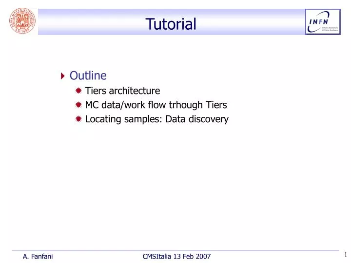
Tutorial. Outline Tiers architecture MC data/work flow trhough Tiers Locating samples: Data discovery. Tiers architecture. Modello di calcolo a Tier di CMS. CMS Tier-0. CMS Tier-0: Accepts data from DAQ Prompt reconstruction Data archive and distribution to Tier-1’s.

E N D
Tutorial • Outline • Tiers architecture • MC data/work flow trhough Tiers • Locating samples: Data discovery
CMS Tier-0 • CMS Tier-0: • Accepts data from DAQ • Prompt reconstruction • Data archive and distribution to Tier-1’s • CAF: CMS Analysis Facility at CERN • Access to full raw dataset • Focused on latency-critical detector trigger calibration and analysis activities • Provide some CMS central services (e.g. store conditions and calibrations)
CMS Tier-1’s • CMS Tier-1 functions: • Real data archiving • Re-processing • Skimming and other data-intensive analysis tasks • Calibration • MC data archiving • CMS Tier-1 resources (average T1 in 2008): • WAN: transfer capacity10 Gb/s • CPU: 2.5 M-SI2k (scheduled reprocessing : analysis = 2 :1) • Disk: 0.8 PB (85% for analysis data serving) • MSS: 2.8 PB
Tier-2’s • CMS Tier-2 functions: • User data Analysis • MC production • Import skimmed datasets from Tier-1 and export MC data • Calibration/alignment • CMS T2 resources (average T2 in 2008): • WAN: 1 Gb/s (at least) • CPU: 900 k-SI2k • Disk: 200 TB
MC Data production • Code working in a CMSSW realease • no prereleases, no patches • Cfg file with convention in PoolOutputModule to describe dataTier module out = PoolOutputModule { ..... untracked PSet datasets = { untracked PSet dataset1 = { untracked string dataTier = “FEVT" } } • An XML file (called workflow file) having all the info to start a production is created • CMSSW release • cfg • input/output dataset names • i.e. /mc-physval-120-ZToMuMu-NoPU/FEVT/CMSSW_1_2_0-FEVT-1167149299 • Convention for LFN namespace that will reflect on storage area organization at sites • /store/mc/2006/12/26/mc-physval-120-ZToMuMu-NoPU/0000/.... • /store/unmerged/mc/2006/12/26/mc-physval-120-ZToMuMu-NoPU/0000/...
Processing Processing Processing ProdAgent basic Workflow Local DBS/DLS • Send Processing jobs to sites • Stage out data at the sites • Report back to ProdAgent • Merge data at site • merge small outputs files produced by individual jobs in fewer larger files • Data registration in local DBS DLS • dataset description (cfg, CMSSW release,...) • extended Framework jobreport used to register files (#evt per file, file size,LFN,...) • Example: • GEN+SIM+DIGI+RECO in 1 step ProdAgent Tier-1 Storage Tier-2 Storage Tier-2 Storage
Processing Processing Processing ProdAgent Workflow reading existing data Local DBS/DLS • Read info about available input data from DBS/DLS • Configure processing jobs to read input data • splitting based on events or on files • The rest is the same as before….. • Example: • DIGI w or w/o PU processing input GEN+SIM • Re-reconstruction on RAW • Skimming on RAW ProdAgent Tier-1 Storage Tier-2 Storage Tier-2 Storage
Making data available CERN Global DBS/DLS Produced data are at sites and registered into DBS/DLS “local” to the ProdAgent • Upload the data to Global DBS/DLS (CMS-wide) Local DBS/DLS ProdAgent • Transfer of the data spread across producing sites to a destination site • PhEDEx : CMS data placement and transfer tool • PhEDEx injection invoked by ProdAgent • Data are available for end user analysis via CRAB
DM concepts • Logical File Name (LFN) - This is a site-independent name for a file. • It doesn't contain either the actual protocol used to read the file or any of the site-specific information about the place where it is located. • you should use this for all production files as then it is possible for a site to change specifics of the access and location without breaking your config file. • A production LFN in general begins with /store and looks like this in a cmsRun cfg file: source = PoolSource { untracked vstring fileNames = { '/store/mc/2006/12/26/mc-physval-120-ZToMuMu-NoPU/0000/guid.root’ }} • Physical File Name (PFN) - This is site-dependent name for a file. • Local access to a file at a site (reading files at remote sites specifying protocol in PFN doesn’t work) • The cmsRun application will automatically convert production LFN's into the appropriate PFN for the site where you are running. So you don't need to know the PFN yourself!! • If you really want to know the PFN, the algorithm that convert LFN to PFN is site dependent and is defined in the so called TrivialFileCatalog at the site. For accessing data locally at CERN you have: • PFN = rfio:/castor/cern.ch/cms + LFN }
Processed dataset - these are just the set of files corresponding to a single sample and produced with a single cfg file • File block - we divide the set of files of a processed dataset up into file blocks. A file block is the minimum quantum of data that we replicate between sites. Each given file block may be at one or more sites.
Discovery page • Search for datasets available on Global DBS/DLS • http://cmsdbs.cern.ch/discovery • http://cmsdbs.cern.ch/discovery_test/