Download
1 / 16
190 likes | 388 Views
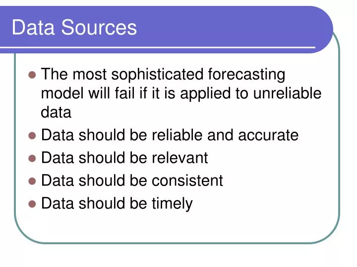
Data Sources. The most sophisticated forecasting model will fail if it is applied to unreliable data Data should be reliable and accurate Data should be relevant Data should be consistent Data should be timely. Forecasting Technique .

E N D
Data Sources • The most sophisticated forecasting model will fail if it is applied to unreliable data • Data should be reliable and accurate • Data should be relevant • Data should be consistent • Data should be timely
Forecasting Technique • Qualitative Forecasting - rely on judgment and intuition - scenario analysis, focus groups, some areas of market research • Quantitative Forecasting - used when historical data is available and the data is judged to be representative of the unknown future. • Statistical techniques - patterns, changes, and fluctuations - decompose data into trends, cycles, seasonality, random • Econometric & Box-Jenkins - do not assume that data are represented by separate components. • Deterministic or causal - identification of relationships (regression)
Types of Data • Cross-sectional: collected at a single point in time – all observations are from the same time period • Time Series – data that are collected, recorded or observed over successive increments of time
Time Series Components • Trend, cyclical, seasonal, random (review Introduction to Forecasting notes for descriptions) • When a variable is measured over time, observations in different time periods are frequently related or correlated. • Autocorrelation - correlation between a variable, lagged one or more periods, and itself. Used to identify time series data patterns.
Autocorrelation • Correlation measures the degree of dependence (or association) between two variables. • Autocorrelation means that the value of a series in one time period is related to the value of itself in previous periods. There is an automatic correlation between the observations in a series. For example, if there is a high positive autocorrelation, the value in June is positively related to the value in May.
Autocorrelation... • Random data? Is there a trend? Stationary data? Seasonal data? • If the series is random, the autocorrelation is close to 0 and the successive values are not related to one another • If the series has a trend, the data and one lag are highly correlated and the correlation coefficients are significantly different from zero and then drop toward zero. • Seasonality - significant autocorrelation occurs at the appropriate time lag: 4 for quarterly, 12 for monthly
95% confidence interval - if autocorrelation is outside the range, have significance Ho: r = 0 HA: r0 Compare T to t-value: 2 tail test, 95% level of significance and n-1 d.f. t-value = 2.2 Reject Ho if T is less than -2.2 or if T is greater than 2.2 Conclusion: Do Not Reject Ho:. The autocorrelation is not significantly different from zero The series is random.
Autocorrelation Analysis • Autocorrelation coefficients of random data have a sampling distribution with a mean of zero and a standard deviation of 1/sqrt(n). • We test to see our data’s autocorrelation coefficients come from a population with the same distribution. If our sample is random, we expect the mean to equal zero. • We use the confidence interval to determine if our autocorrelation coefficients are within a certain range of zero, based on the standard deviation
Autocorrelation Analysis • If the series has a trend, the data is non-stationary. Advanced forecasting models require stationary data - average values do not change over time. • Autocorrelation coefficients drop to zero after the second time lag in stationary data. • Can remove a trend from a series by differencing (subtract the lagged data from original data) and check the correlogram to make sure the data does not show a trend.
Choosing a Forecasting Technique • Stationary data • Can transform stationary data - square roots, logs, differences • Forecasting errors can be used in simple models • Adjusting data for factors such as population growth • Simple models: averaging, simple exponential smoothing, naive
Choosing a Forecasting Technique • Forecasting Trends • Growth or decline over extended time-period • Increased productivity / changes in technology / population / purchasing power • Models: linear moving average, exponential smoothing, regression, growth curves
Choosing a Forecasting Technique • Forecasting Seasonality • Repeated pattern year after year • Multiplicative or additive method and estimating seasonal indexes • Weather or calendar influences • Models: classical decomposition, multiple regression, time series & Box-Jenkins
Other factors to consider • Selection depends on many factors - content and context of the forecast, availability of historical data, degree of accuracy desired, time periods to be forecast, cost/benefit to the company, time & resources available. • How far in the future are you forecasting? Ease of understanding. How does it compare to other models? • See Table in Text • Forecasts are usually incorrect (adjust) • Forecasts should be stated in intervals (estimate of accuracy) • Forecasts are more accurate for aggregate items • Forecasts are less accurate further into the future
^ Y ^ ^ Yt Yt Yt - Forecasting Error • Some symbols: Actual Value Y Forecasted Value Forecasted Value for time period t et = residual or forecast error =
Forecast Errors • MAD measures forecast accuracy by averaging the absolute value of the forecast errors (n = number of errors and not sample size). Magnitude of errors. • MSE (Mean Squared Error) - each error is squared, then summed and divided by the number of observations (errors). Identifies large forecasting errors because of the squares • MAPE (Mean absolute percentage error) - percentages. Find the MAD for EACH period then divide by actual of that period and dividing the sum by the number of errors. How large the forecast errors are in comparison to the actual values. • MPE (Mean percentage error) - determines bias (close to 0 is unbiased; - is overestimating; + is underestimating)
Technique Adequacy • Are the autocorrelation coefficients of the residuals random? • Calculate MAD, MSE, MAPE, & MPE • Are the residuals normally distributed? • Is the technique simple to use?