Download
1 / 52
520 likes | 623 Views
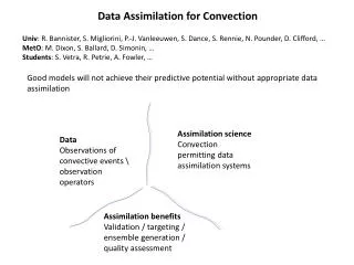
Data Assimilation for the Space Environment. Ludger Scherliess. Center for Atmospheric and Space Sciences Utah State University Logan, Utah 84322-4405 GEM 2003 Meeting Snowmass, CO June 2003. Data Assimilation. Create a coherent and objective ‘picture’ of the space

E N D
Data Assimilation for the Space Environment Ludger Scherliess Center for Atmospheric and Space Sciences Utah State University Logan, Utah 84322-4405 GEM 2003 Meeting Snowmass, CO June 2003
Data Assimilation • Create a coherent and objective ‘picture’ of the space • environment by combing the information inherent • in the physical model and in the data. • This ‘picture’ (analysis) should satisfy the physical • laws and fit the data as best as possible (within their • errors). • The analysis can than serve as the best initial • condition for a forecast.
Historical Background • Data Assimilation in the Atmosphere: • Initial Attemps started in the 1950th (NWP) • Currently adjoint/variational methods are used • Used now also in re-analysis runs to get consistency • for the past 40 years. • Data Assimilation in the Oceans: • Began with large scales (mean properties) • Regional effords (e.g., Gulf stream) [10-15 yrs ago] • El Nino, emphasis on equatorial pacific (coupled • with atmosphere) • GODAE, produce operational upper ocean now- and • forecast.
Data Assimilation in Space Sciences • Assimilative Mapping of Ionospheric Electrodynamics • (AMIE, Richmond and Kamide, 1988) • Initial Testing of Kalman Filter for Ionospheric Electron • Density Reconstructions (Howe et al., 1998) • Kalman Filter to construct the global 3-D Electron Density • Field (GAIM) Until Recently only relatively Sparse Data were available
Global Assimilation of Ionospheric Measurements (GAIM) • Multi-University Research Initiative (MURI): • Utah State University (PI R. W. Schunk) • University of Colorado - Boulder • University of Texas at Dallas • University of Washington Basic Approach: Use a Physics-Based Ionosphere-Plasmasphere Model as the Basis for Assimilating a Diverse Set of Real-Time (or Near Real-Time) Measurements.
Motivation • Data Assimilation has been proven very successful in • Meteorology and Oceanography • Need for More Accurate Now-Casting and Forecasting of • Plasma Distribution in the Ionosphere and Plasmasphere • (and Magnetosphere?) • Availability of Large Quantities of Data • Diverse Data Sources (Apples and Oranges) • Mature Theoretical/Numerical Space Environment Models • Models contain our ‘knowledge’ of the physics • Data contain information about the ‘true’ state
Objectives • Goal: Optimally combine Data and the Model to create • coherent Picture of the Space Environment • Solution satisfies the physical laws and ‘agrees’ with the data • (within their error bounds) • Both, however, are imperfect: • Models: Forcing, Parametrization, etc. • Data: Observational Errors
Data Collection Quality Control ‘Best-Guess’ Background Short-Term Forecast Analysis Forecast The Data Assimilation Cycle Physical Model creates a forecast which is adjusted by the Data to create an ‘analysis’, which serves as the start for the next model forecast. In the analysis the Data Errors and Model Errors are used as weights.
Data Assimilation Techniques • 3-d Var • 4-d Var • Kalman Filter • xf = Mx + • Pf = MPMT + Q • yo = Hx + • K = PfHT (HPfHT + R)-1 • xa = xf + K(yo - Hxf) • Pa = (I-KH)Pf
Fundamental Concept of 3D-Var • Start with a forecast of the physical model. • Produce an analysis by minimizing the difference between • the analysis and a weighted combination of • the forecast (the background or best guess field) and • the observations. • At each time-step take a ‘snapshot’ of the state • This ‘snapshot’ will serve as the initial condition for the next forecast. • We want to minimize a “Cost Function” J which consists of: • J = JB + JO +JC
The Cost Function • J= JB+JO+ JC • JB: Weighted fit to the background field • JO: Weighed fit to the observations • JC: Constraint which can be used to impose • physical properties (e.g., analysis should satisfy • Maxwell’s equations, continuity equation, …) • Strong Constraint: Exactly satisfied • Weak Constraint: Approximately satisfied
The Cost Function, cont. • A typical form for the JB term is: • JB = (xA - xB)T B-1 (xA - xB) • Where: • xA: Analysis Variable (e.g., Electron Density,Temperature,…) • xB: Background Field, obtained from the Model Forecast • B : Background Error Covariance Matrix: • How good is your Forecast: • Good Forecast high weight • Poor Forecast low weight
The Cost Function, cont. • A typical form for the JO term is: • JO = [y - H(xA)]T R-1 [y - H(xA)] • Where: • y : Represents all Observations • H : Forward Operator which maps the Grid Point Values to • Observations (can be linear or nonlinear) • R : Observation Error Covariance Matrix: • Make use of the probable Errors of the Data • Good Data high weight • Poor Data low weight • (also includes the representativeness of the data) Constantly compares the data with the model
The Cost Function, cont. • Analysis is found my minimizing J using “standard minimization techniques” (find the gradient of J). • The analysis is found by: • Analyzing all points at once • Using all available data • The Physical Properties/Model were used to: • Obtain the best possible background field • To constrain the Analysis • Cost function and the constraints are not explicitly time dependent
Fundamental Concepts of 4D-Var 4D-Var introduces the temporal dimension to data assimilation • Find a close fit to the data that is consistent with the • dynamical model over an extended period of time. • Find the the closest trajectory Physical model • 4D-Var is a powerful technique to find: • Initial conditions • External Forcing
The Kalman Filter In the Kalman filter the weight for the background (error covariance matrix) evolves with the same physical model as the state! • x - Model State Vector • M - State Transition Matrix • - Transition Model Error • P - Model Error Covariance • Q - Transition Model Error Covariance • y - Data Vector • H - Measurement Matrix • - Observation Error • R - Observation Error Covariance • K - Kalman Gain
Kalman Filter Equations • x - Model State Vector • M - State Transition Matrix • - Transition Model Error • P - Model Error Covariance • Q - Transition Model Error Covariance • y - Data Vector • H - Measurement Matrix • - Observation Error • R - Observation Error Covariance • K - Kalman Gain Model-State Forecast
Kalman Filter Equations • x - Model State Vector • M - State Transition Matrix • - Transition Model Error • P - Model Error Covariance • Q - Transition Model Error Covariance • y - Data Vector • H - Measurement Matrix • - Observation Error • R - Observation Error Covariance • K - Kalman Gain Model-State Forecast Error
Kalman Filter Equations • x - Model State Vector • M - State Transition Matrix • - Transition Model Error • P - Model Error Covariance • Q - Transition Model Error Covariance • y - Data Vector • H - Measurement Matrix • - Observation Error • R - Observation Error Covariance • K - Kalman Gain Measurement Equation
Kalman Filter Equations • x - Model State Vector • M - State Transition Matrix • - Transition Model Error • P - Model Error Covariance • Q - Transition Model Error Covariance • y - Data Vector • H - Measurement Matrix • - Observation Error • R - Observation Error Covariance • K - Kalman Gain Kalman Gain
Kalman Filter Equations • x - Model State Vector • M - State Transition Matrix • - Transition Model Error • P - Model Error Covariance • Q - Transition Model Error Covariance • y - Data Vector • H - Measurement Matrix • - Observation Error • R - Observation Error Covariance • K - Kalman Gain Model-State Analysis
Kalman Filter Equations • x - Model State Vector • M - State Transition Matrix • - Transition Model Error • P - Model Error Covariance • Q - Transition Model Error Covariance • y - Data Vector • H - Measurement Matrix • - Observation Error • R - Observation Error Covariance • K - Kalman Gain Model-State Analysis Error
The Dynamical Model entered the Filter: • Evolution of the State Vector (make a Forecast) • Evolution of the Error Covariance Matrix • Error Covariance Matrix becomes time-dependent! • Model Error is explicitly included in the Assimilation
Data Assimilation Tasks • Develop Physical Model • Develop Assimilation Algorithm • Data Acquisition Software • Data Quality Control • Executive System • Validation Software
Kalman Filter Example Electron Density Along Field Line • Kalman Filter with synthetic data • Truth generated with IFM with • Modified equatorial drift • 1 Ne Measurement every 15 min at • magnetic equator Kalman Truth Climat Observation
Kalman Filter Example Electron Density Along Field Line • Kalman Filter with synthetic data • Truth generated with IFM with • Modified equatorial drift • 1 Ne Measurement every 15 min at • magnetic equator Kalman Truth Climat Observation
Kalman Filter Example Electron Density Along Field Line • Kalman Filter with synthetic data • Truth generated with IFM with • Modified equatorial drift • 1 Ne Measurement every 15 min at • magnetic equator Kalman Truth Climat Observation
Kalman Filter Example Electron Density Along Field Line • Kalman Filter with synthetic data • Truth generated with IFM with • Modified equatorial drift • 1 Ne Measurement every 15 min at • magnetic equator Kalman Truth Climat Observation
Kalman Filter Example Electron Density Along Field Line • Kalman Filter with synthetic data • Truth generated with IFM with • Modified equatorial drift • 1 Ne Measurement every 15 min at • magnetic equator Kalman Truth Climat Observation
Next, consider the more complicated situation: • Global Reconstruction • Many observations • Different kinds of instruments measuring different • quantities • Observations are in different places
Data Distribution We currently assimilate data from 16 globally distributed DISS Stations and more than 100 GPS Ground Stations. The GPS Stations are linked to the Fleet of GPS Satellites. In addition, we assimilate Electron Density Data from two DMSP Satellites and simulated data from the C/NOFS satellite in the Filter.
A Model TID • In this “test,” the following are variables • TID Equatorward Speed • TID Width in Latitude • TID Amplitude History • In this “test,” the assumptions are • TID is a perturbation on the background ionosphere. • TID perturbed densities are very noisy • TID moves along a meridian. • Observations lie along the meridian. • Propagation with simple advective model
1-D TID/TAD • 1-D Propagation • Propagation along meridian • Density Perturbations • Network of ~10 observatories
1-D TID/TAD • 1-D Propagation • Propagation along meridian • Density Perturbations • Network of ~10 observatories
1-D TID/TAD • 1-D Propagation • Propagation along meridian • Density Perturbations • Network of ~10 observatories
1-D TID/TAD • 1-D Propagation • Propagation along meridian • Density Perturbations • Network of ~10 observatories
The Observations • 10 Stations • Density Perturbations • 100% Noise
Kalman Filter Reconstruction • Reconstruction of TID Density Perturbations • # of Stations = 10 • 100% Noise • True Velocity = 2 T=1
Kalman Filter Reconstruction • Reconstruction of TID Density Perturbations • # of Stations = 10 • 100% Noise • True Velocity = 2 T=2
Kalman Filter Reconstruction • Reconstruction of TID Density Perturbations • # of Stations = 10 • 100% Noise • True Velocity = 2 T=3
Kalman Filter Reconstruction • Reconstruction of TID Density Perturbations • # of Stations = 10 • 100% Noise • True Velocity = 2 T=4
Kalman Filter Reconstruction • Reconstruction of TID Density Perturbations • # of Stations = 10 • 100% Noise • True Velocity = 2 T=5
Kalman Filter Reconstruction • Reconstruction of TID Density Perturbations • # of Stations = 10 • 100% Noise • True Velocity = 2 T=6
Kalman Filter Reconstruction • Reconstruction of TID Density Perturbations • # of Stations = 10 • 100% Noise • True Velocity = 2 T=10
Kalman Filter Reconstruction • Reconstruction of TID Density Perturbations • # of Stations = 10 • 100% Noise • True Velocity = 2 T=15
Kalman Filter Reconstruction • Reconstruction of TID Density Perturbations • # of Stations = 10 • 100% Noise • True Velocity = 2 T=20
Kalman Filter Reconstruction • Reconstruction of TID Density Perturbations • # of Stations = 10 • 100% Noise • True Velocity = 2 • Guessed Velocity • 50% Off
Kalman Filter Reconstruction • Reconstruction of TID Density Perturbations • # of Stations = 10 • 100% Noise • True Velocity = 2 • Guessed Velocity • 50% Off