Download
1 / 23
240 likes | 326 Views
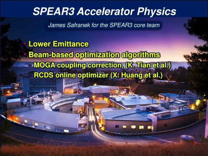
SPEAR3 Accelerator Physics. James Safranek for the SPEAR3 core team Lower Emittance Beam-based optimization algorithms MOGA coupling correction, (K. Tian et al.) RCDS online optimizer (X. Huang et al.). Emittance Reduction (4.380 M$, FY13-15).

E N D
SPEAR3 Accelerator Physics James Safranek for the SPEAR3 core team Lower Emittance Beam-based optimization algorithms MOGA coupling correction, (K. Tian et al.) RCDS online optimizer (X. Huang et al.)
Emittance Reduction (4.380 M$, FY13-15) Cost (k$) 4380 ? x’ x • Effective emittance, ex,eff includes hx:
Brightness (500 mA) Brightness improvement: (x3, ex)(x5, current)(top-off) = x20 total
Injection optimization for lower ex • Reduce septum wall width • 6.3 mm to 2.5 mm • Upgrade K2 injection kicker pulser • Improve dynamic aperture • Increase number of sextupole power supplies from 4 to 10 • Individual supplies too costly • MOGA optimization • Improve control of injected beam • (Reduce injected beam emittance) Arc cell: QFC QD QD QF QF BEND BEND SD SF SF SD
Benefit of additional sextupole power supplies log10(turns) Dynamic aperture improved Sextupole strength distribution
Experiments with lower ex lattice • 20% injection efficiency • Corrected linear optics (LOCO), ey = 4 pm • Measurement of chromaticity (w/ high order) • Energy acceptance • 3nx resonance characterization • Injection rate vs. tune scan • Measurement of detuning coefficients 6 hour lifetime ey = 8 pm 500 mA
Automated beam-based optimization • Motivation • USR designs fine-tuned with detailed analytical and computational optimization • As built machines are never exactly as designed • Need to develop detailed beam-based optimization • Techniques • K. Tian et al. (to be published) • Genetic optimization • Minimize ey • Maximize measured beam loss as function of 13 skew quadrupoles • X. Huang et al. (NIMA 726, 2013) • New optimization algorithm, RCDS (robust conjugate direction search) • Tested in simulation and online • Optimization of injection efficiency, coupling, kicker bump matching
Beam Loss Rates and CouplingK. Tian et al. By inserting the horizontal scraper, we collect most of the touschek beam loss at one location. A simple scaling for beam loss rates, beam size, and the linear coupling is (assuming εxand σx are constant): Experimental Verification: 1/sy (1/mm) coupling (%) DCCT loss rate (A.U.) loss monitor (counts/s) loss monitor (counts/s) Minimize Coupling Maximize Loss Rates
Machine Based GA for Maximizing Beam Loss RateK. Tian et al. Decision Variables: 13 skew quads Objective Functions: Measured Beam Loss Rates Population size: 120 Genetic Operators: real-coded Simulated Binary Crossover (SBX) and polynomial mutation normalized beam loss (cnts/mA2) current (A) 220 generations for over 9 hours time (s) skew quadrupole Comparison of linear coupling and beam loss:
Robust Conjugate Direction Search, RCDS X. Huang et al. • Fast, minimize objective evaluations • Robust – surviving noise, outliers and machine failures • Algorithms considered: • Gradient based method are not considered because of noise. • Iterative 1D scan (that automates manual tuning procedure) • Nelder-Mead (downhill) simplex method • MOGA (Not efficient). • Powell’s conjugate direction method • Robust conjugate direction method (RCDS) – A combination of Powell’s method and a new noise resistant line optimizer.
Parameter scan and simplex methods Iterative parameter scan may be inefficient. In a common situation depicted above, each x- or y-scan makes a tiny step downward*. Simplex method may fail to reach the optimum when noise starts to change results of vertex comparison. *W.H. Press, at al, Numerical Recipes
The robust line optimizer objective Initial solution conjugate variable Step 1: bracketing the minimum with noise considered; scan until Obj-Objmin > 3s Step 2: Fill in empty space in the bracket with solutions and perform quadratic fitting. Remove any outlier and fit again. Find the minimum from the fitted curve. Global sampling within the bracket helps reducing the noise effect. RCDS is Powell’s conjugate method* + the new robust line optimizer. *however, since the online run time is usually short, it is important to provide a good initial conjugate direction set which may be calculated with a model.
RCDS tests – simulation and experiments • Simulation • SPEAR3 coupling • Transport line optics • Experiments • SPEAR3 coupling • Kicker bump match • Injected beam steering • Transport line optics coupling ratio RCDS fast & effective #objective evaluations b-oscillation (mm) -DCCT loss rate (mA/min) #objective evaluations #objective evaluations
The Matlab RCDS package • The RCDS algorithm is implemented in Matlab. • Features • Each parameter has a specified range, i.e., the parameter space is bounded. This is important for online application. • The parameter space is normalized to a hyper unit cube (each parameter normalized to [0, 1]). • Optimization algorithm is decoupled from the specific application. Application to a new problem is done by defining the objective function. Users need not to look into the algorithm. • Data are saved in Matlab global variable space and won’t get lost (unless Matlab crashes). This package is available.
Summary • Plans to reduce SPEAR3 emittance to 6 nm • 1020 brightness • Probably close to limit for SPEAR3 geometry • 5 nm with S.C. damping wigglers • Ideas? • Beam-based optimization algorithm development • MOGA coupling correction, (K. Tian et al.) • Publication soon • RCDS online optimizer (X. Huang et al.) • NIMA 726, 2013 • Code available (ask Xiaobiao)
Comparison of performance (best of 6-s cases) The IMAT method uses the same RCDS line optimizer, but keep the direction set of unit vectors (not conjugate). Clearly, the line optimizer is robust against noise. Searching with a conjugate direction set is much more efficient. Note that the direction set has been updated only about 8 times after 500 evaluations (out of 13 directions). So the high efficiency of RCDS is mostly from the original direction set.
Transport line optics • BTS transport line optics matching • Varying 6 quads in BTS for optics matching between transport line and storage ring. • Noise is generated from the finiteness of the number of particles. With 1000 particles in a distribution, the noise sigma of injection efficiency is 1.6%. • Initial conjugate direction set is from SVD of beam moments (elements of the -matrix) w.r.t. quads. • Dynamic aperture of the ring is intentionally shrunk to 12.5 mm in the simulation.
Coupling correction with loss rate Beam loss rate is measured by monitoring the beam current change on 6-second interval (no fitting). Noise sigma 0.04 mA/min. Data were taken at 500 mA with 5-min top-off. Initially setting all 13 skew quads off. Loss rate at about 0.4 mA/min. Final loss rate at about 1.75 mA/min. At 500 mA, the best solution had a lifetime of 4.6 hrs. This was better than the LOCO correction (5.2 hrs) On a later shift (5/6/2013), with 6-s DCCT data fit for loss rate, loss rate reached >2.0 mA/min at 500 mA and lifetime was 4.2 hrs.
Coupling correction with pinhole camera Sigmay noise level at 0.3 micron. All 13 skew quads were off initially. Experiments were done with septum off (while beam loss-based experiments were with septum on). The operation lattice (with lifetime 8.4 hrs at 500 mA) has a vertical beam size of sigmay = 20 um. The best solution from this run had sigmay = 13 um.
Kicker bump matching Parameters: Adjusting pulse amplitude, pulse width and timing delay of K1 and K3 (with K2 fixed) and two skew quads for vertical plane (This is the setup by James for kicker bump matching), 8 parameters total. Objective: sum of rms(x) and rms(y) of turn-by-turn orbit (for 30~300 turns). First time of getting kicker bump for low alpha lattice matched. The LA20 lattice matching was further improved on a second shift.
Injected beam steering for SPEAR3 Use four end steering magnets in the BTS transport line to steer the injected beam. The objective function is injection efficiency. Low betay lattice Injection efficiency noise level: sigma=1%. Low betay lattice
BTS optics For injection optics matching, ideally we need to decouple the steering effect of quadrupole changes (when beam trajectory is off-center). But we haven’t done that yet. To test the algorithm, we changed the 9 BTS quads setpoints randomly to mess up injection and use the code to bring injection back. Knobs: 9 BTS quads. Objective: injection efficiency.