Download

1 / 60
600 likes | 796 Views
CHEE 370 Waste Treatment Processes. Last Lecture Final Exam Review. Wastewater Constituents. Suspended solids Biodegradable organics Micro-organisms Nutrients Refractory organics Heavy metals Dissolved inorganics Physical contaminants (temperature, colour, odour, solids).

E N D
CHEE 370Waste Treatment Processes Last Lecture Final Exam Review
Wastewater Constituents • Suspended solids • Biodegradable organics • Micro-organisms • Nutrients • Refractory organics • Heavy metals • Dissolved inorganics • Physical contaminants (temperature, colour, odour, solids)
Evaporation and drying at 105 ºC Measurement of Solids Evaporation and drying at 105 ºC Ignition at 500 ºC TS = TVS + TFS TS = organic + inorganic 2.3 Metcalf & Eddy
The BOD Test COHNS + O2 + bacteria (C5H7NO2) more C5H7NO2 + CO2 + H2O + NH3 + other • An INDIRECT measure of the organic content • Measures the amount of oxygen consumed as the bacteria found in the WW use the organic material as a carbon/energy source for the production of more bacteria BODt=UBOD(1 - e-kt)
Chemical Oxygen Demand (COD) • An INDIRECT measure of the organic content • Mass of oxygen theoretically required to completely oxidize an organic compound to carbon dioxide • Measured by mixing the WW with a very strong chemical oxidant CODin = CODout + O2consumed
Total Organic Carbon (TOC) • A DIRECT measure of the organic content • In theory - based on the chemical formula • In practice - organic carbon is converted to carbon dioxide, which can then be measured Theoretical Oxygen Demand (ThOD) • An INDIRECT theoretical measure of organic content • Calculated using stoichiometric equations • Considers both carbonaceous and nitrogenous oxygen demand
Additional Characterization • Micro-organisms • Total coliform, fecal coliform • Toxicity • Acute toxicity (LC50), Chronic toxicity • Nutrients • TKN, NH3, TP, ortho-phosphate • Flowrates • Hydraulic flowrates (peak and min), Loadings
Screening - Headloss • hL = headloss (m) • C = empirical discharge coefficient to account for turbulence and eddy losses (clean screen = 0.7; clogged screen = 0.6) • V = velocity through the openings (m/s) • v = approach velocity in upstream channel (m/s) • g = acceleration due to gravity (9.81 m/s2)
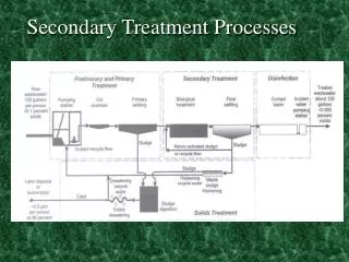
Types of Settling • Type I: Discrete Settling • Type II: Flocculent Settling • Type III: Hindered or Zone Settling
Type I Settling Discrete Settling • Settling of discrete, non-flocculating particles • Found in grit removal tanks! • Particles settle as individual entities at a constant velocity • Minimal interaction between particles • Applies only to particles in a suspension with a low solids concentration
Type I SettlingCritical Settling Velocity • vo= critical settling velocity • A particle starting at the top of the inlet zone with a settling velocity of vo will just reach the bottom of the tank at the beginning of the outlet zone
Type I SedimentationAnalysis • Use a batch settling column • Withdraw samples from a fixed height “h” at time intervals and measure the solids concentration • Calculate the weight fraction remaining • Calculate the settling velocity for the particles at each of the time intervals (vs = h/t) • Plot the weight fraction remaining versus velocity (cumulative distribution curve)
Type II SettlingFlocculant Particle Settling • Particles coalesce as they settle • Rate of settling (vs) changes with time • Particles change in size, shape and weight as they settle • Larger particles have a higher vs
Type II SettlingAnalysis • Use a batch settling column with multiple sampling ports • Withdraw samples from each port at time intervals and measure the solids concentration • Calculate the weight fraction removed • Prepare a plot of sampling depth versus time and indicate the weight fraction removed for each of the samples • Draw the “equal percent removal” lines at intervals of 10% on the plot
r3 r2 r1
Type I and Type II SettlingClarifier Dimensions • A = L x W = surface area of the basin (m2) • Default aspect geometry: • L = 4W • A = 4W2
Type I and Type II SettlingScouring Velocity • Re-suspension of particles due to large horizontal velocities (u) • Where: • u = horizontal velocity (m/s) • Q = water flowrate (m3/s) • HW = cross-sectional area (entry area) in the direction of flow (m2) To prevent scouring, u < (9 * vo)
Type III SettlingHindered or Zone Settling • Occurs in solutions with a very high solids concentration • Strong cohesive forces between the particles cause them to settle collectively as a zone • Distinct interface between the settled particles and the clarified effluent
Type III SettlingClarifier Design • Secondary clarifiers need to be designed for two purposes: • Clarification • Thickening
Type III SettlingSecondary Clarifier Design • Calculate the area required for clarification • Where: • vo = initial zone settling velocity at the feed concentration (X), [m/h], (function of X) • Ac = surface area for clarification [m2] • Qe = overflow rate of clarified liquid [m3/h]
Type III SettlingSecondary Clarifier Design • Calculate the area required for thickening • Find the gravity mass flux • Where: • Gg = gravity flux [M/L2•T] (kg/(m2•h)) • vi = settling velocity at solids concentration Xi [L/T] (m/h) • Xi = local concentration of solids [M/L3] (kg/m3)
Type III SettlingSecondary Clarifier Design • Calculate the area required for thickening • Find the bulk mass flux due to underflow pumping • Where: • ub = bulk downward velocity of the solids [L/T] (m/h) • Qu = underflow flowrate [L3/h] (m3/h) • A = surface area of settling tank [L2] (m2)
Type III SettlingSecondary Clarifier Design • Calculate the area required for thickening • Find the total mass flux • Plot G, Gg, Gu
Type III SettlingSecondary Clarifier Design • Identify which area is greater: • Area for clarification • Area for thickening • Use the larger area to size the clarifier • Adesign = 1.75*Acalculated • For an ideal clarifier, L = 4W
Designing for a Specific Underflow Solids Concentration (Not Given ub)
Batch Bacterial Growth Curve • Lag Phase • Acclimation to environment • Exponential Growth Phase • Multiplication at max rate • Rapid utilization of S • Stationary Phase • Growth is offset by death • Steady state • Death Phase • Depletion of S • Decrease in X due to cell death Metcalf and Eddy; Figure 7-10
WW TreatmentBacterial Growth Rate • Where: • X = biomass concentration (mass/volume) • = specific growth rate (time-1) • kd = endogenous decay coefficient (time-1)
Bacterial Growth in Biological WW TreatmentMonod Kinetics • Specific growth rate increases as the concentration of the limiting substrate S increases • = specific growth rate (time-1) • max = maximum specific growth rate (time-1) • S = concentration of the growth limiting substrate (M/V) • Ks = half saturation constant (M/V)
Michaelis-Menten Continued • Derivation carried out in class! • Now analogously, if our “product” are cells the above specific rate of cell formation is as described as:
Estimation of Kinetic Parameters • It is possible to estimate the kinetic parameters (Ks, kd, max, Y) from bench-scale CSTR process data in order to design biological waste treatment facilities • Perform tests starting with a known limiting substrate concentration So • Measure X and S at various residence times ()
CSTR With No Recycle Problems • If the kinetic parameters (Ks, kd, max, Y) are known, and you are given So, Q, and one additional variable (i.e. S, U, V), then you can solve for the rest
COD Mass BalanceOxygen Consumed • When working in COD units, you can always perform a mass balance COD substrate in = COD substrate out + COD biomass out + O2 consumed O2 consumed = COD substrate in - COD substrate out - COD biomass out O2 consumed = COD substrate consumed - COD biomass out
Conversion Factor (f) • Required to determine the oxygen requirements if the substrate concentration is expressed in terms of BOD5 • If you are given the influent substrate concentration in terms of BOD5 and UBOD, you can calculate “f” to determine the effluent substrate concentration in UBOD units
AS - Aeration Requirements • Air supply requirements can be expressed in a variety of units • kg O2/day, kmol O2/day, m3 O2/day, m3 air/day • Conversion factor: 22.4 m3 gas/kmol (@ STP) • Air contains ~21 % O2 • If the oxygen transfer efficiency of the aeration system is known or can be estimated, the air requirements may be determined ALWAYS DESIGN AERATION SYSTEMS WITH A SAFETY FACTOR OF 2
SVI Determination • Take a sample of MLSS from the aeration basin • Settle for 30 min (usually in a 2 L container with a diameter larger than a graduated cylinder) • Determine the volume and mass of the settled solids Y, settled volume of sludge (mL) X, mass of settled solids (g) Typical range: 50 - 150 mL/g Units of mg/L
TF Design Equation • z = depth of the packing media/bed [ft] • Q = applied flow (Qo + Qr) [MG/D] • A = filter bed cross-sectional area = π•r2 [Acres] • n, K = constants; f(packing media); • See table 6.11
AD Model Assumptions • Design based on the rate-limiting step - breakdown of volatile fatty acids (VFAs) • Non-biodegradable fractions of COD remain unchanged by the digestion process • Heterotrophic bacteria only decays and the COD associated with decay will be accumulated as VFAs available to the methanogens • Complete hydrolysis and fermentation of biodegradable organic matter -> fully available to methanogens • Use the kinetics for the growth of the methanogens to determine the minimum SRT, then use this value with a safety factor to determine the operating conditions
Minimum SRT Calculation • Where: • umax,m = maximum specific growth rate for the methanogens • Kd,m = decay rate for the methanogens
Factor of Safety for Growth • It is necessary to provide a factor of safety for methanogen growth (prevent “stuck” digester) and headspace • Use a factor of safety of at least 2.5 • The ministry of the environment requires at least 15 days SRT at 35 C • Compare with your calculation and select the larger value
Heterotroph Mass Balance • Assume there is no growth - only decay • Perform a mass balance on the digester for the heterotrophic bacteria: • As the SRT increases, the amount of active heterotrophic biomass in the effluent decreases
Debris Mass Balance • Debris (XD) can enter the digester in the influent (XDo) stream and is also generated during biomass decay • Perform a debris mass balance on the digester : • Where fd = debris fraction of the degraded biomass (fd ranges from ~ 0.08 - 0.20)
VFAs for Methanogens • Multiple Sources: • Soluble biodegradable COD (Ss) • Biodegradable particulate COD (Xs) • Decay of heterotrophic biomass
Effluent VFA and Formation of Methanogenic Bacteria • CSTR without recycle
Methane Production • COD balance can be performed in order to determine the amount of methane produced • CODin = Q(SSo + XSo + XHo + XDo) • CODout = Q(Svfa + XH + Xm + XD) CODin = CODout + CODmethane produced CH4 + 2O2 CO2 + 2H2O • 64 g COD/mol CH4