Download
1 / 14
140 likes | 259 Views
Occupation / queue size. D/D/1 : Constant arrivals, constant duration. M/D/1 : Exponential arrivals, constant duration. queue size. 4a. 2a. a. occupation rate. 0.6. 0.8. 0.9. 1. Arena experiments. M/D/1 queues. D/D/1 queues. Tandem queues. Assignment 2.

E N D
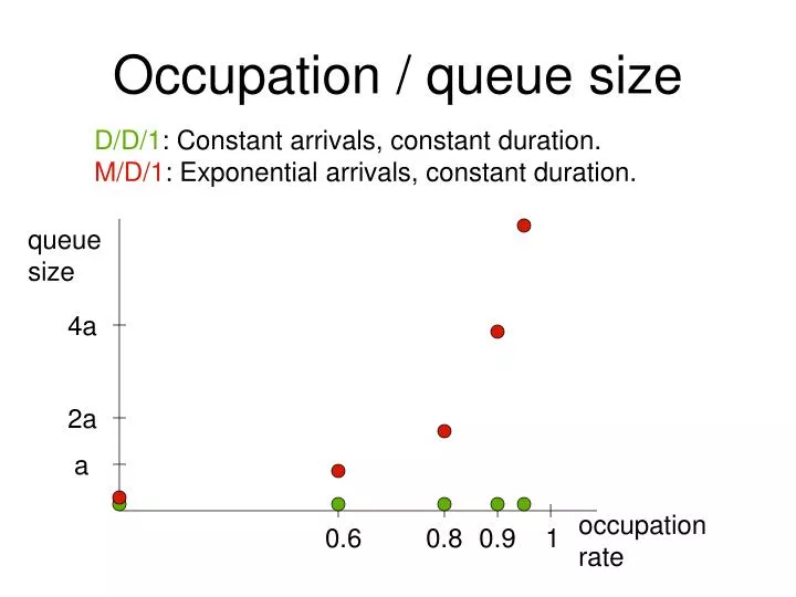
Occupation / queue size D/D/1: Constant arrivals, constant duration. M/D/1: Exponential arrivals, constant duration. queue size 4a 2a a occupation rate 0.6 0.8 0.9 1
Arena experiments M/D/1 queues. D/D/1 queues. Tandem queues.
Assignment 2 Goal: obtain Arena knowledge. Modeling+experimenting. Various models are possible. Several modeling pitfalls. Use of expression builder. Repeated test vs. "hold" block.
Modeling: parameter choice Problem definition Conceptual impl: Arena CPN Tools Modeling parameterization Validation Experiment Interpret
Modeling: parameters Parameters for a model obtained by a combination of - observations (direct / video recordings), - event logs (e.g. SAP): often interpretation needed, - interviews. Select a distribution that accords with theory and matches measured averages. Example: "create" block M measured arrivals in N time units; exponential distribution with intensity M /N.
DCT arrivals Import trace into spreadsheet. DCT trace: arrival 1 at 0.00, 500 at 687.835. exp., avg interarrival time 687.835 / 499. Model should differentiate between B/F/BF trucks: three generators with three different intensities. Intensities may stay the same or fluctuate. first 108 B trucks 0-265, next 108 265-678 first 49 BF trucks 13-363, next 49 368-681 first 90 F trucks 1-427, next 90 427-686. There may be reasons for fluctuations (e.g. traffic); look for confirmation by interviews!
Arena input analyzer Trace file is imported into spreadsheet and sorted. Export selected data to text file, which can be read by input analyzer. Example with interarrival times for B trucks. However, no variable-intensity exponential distribution. So, divide in subparts and analyze separately. Keep asking questions! Listen to answers given!
Processing times Inferring processing times from trace. Problem with assessing duration for steps needing resources. Suppose step needs a resource R. Job id start B rdy B 123 8.79 10.01 127 11.26 13.10 136 13.24 14.67 132 14.87 16.25 Idle time of R in between? Look at predecessor job(s)!
Assess resource occupation Job id rdy A start B rdy B 123 8.58 8.79 10.01 127 11.13 11.26 13.10 136 12.09 13.24 14.67 132 13.12 14.87 16.25 When is resource R idle? Apparently, R not immediately available after rdy B.
1.38 1.43 1.22 1.84 0.13 ? ? 0.21 0.14 ? ? 0.20 Resource usage modeling Job id rdy A start B rdy B 123 8.58 8.79 10.01 127 11.13 11.26 13.10 136 12.09 13.24 14.67 132 13.12 14.87 16.25 A2B st B rdy B rdy A B-queue empty ↔ t can be timed ↔ u cannot be timed
30(BF) 31(B) 32(B) ...... 44(BF) 42(B) 43(F) 45(B) 46(BF) DCT processing Important for keeper occupation: arrival (ar), start (sk), error (er), approved (ap), fail (fl). extra keeper occupation
Keeper process Keeper busy time(ap) - time(sk) + plm. 0.07 if OK time(er) - time(sk) + plm. 0.07 if failure time(er) - time(sk) + ?(extra) if corrected Assumption: extra time equals normal check time
DCT processing Important for crane occupation: mv/d, s1/2, gt/p, pt/p, rd. 19(B) 21(B) 24(B) 0.23 25(B) 0.21 0.19 20(BF) 22(F) 23(F)
Crane process Six different paths: B, F, BF, with and without extra first move. F and BF have an optional s1/s2 step for obtaining the needed container. Two modeling options: 1. Model each step; fit distributions for each step. Do not forget the extra time after "pp" step. 2. Aggregate and use a bit of analysis to approximate distribution(s). Simulation can be used to find out whether option 2 is appropriate.