Download
1 / 60
600 likes | 804 Views
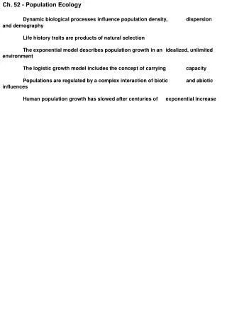
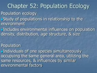
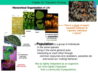
Chapter 52 Population Ecology. Population Ecology. Study of Populations in relation to their environment. Environmental influences on Pop. Density Distribution Age structure size. Individuals of a single species that occupy the same general area. Population:.

E N D
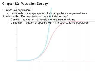
Chapter 52 Population Ecology
Population Ecology • Study of • Populations in relation to their environment. • Environmental influences on • Pop. Density • Distribution • Age structure • size
Individuals of a single species that occupy the same general area. Population:
Important Characteristics • Density 2. Dispersion
Density • Number of individuals per unit area or volume. • Ex: • Diatoms - 5 million/m3 • Trees - 5,000/km2 • Deer - 4/km2
Dispersion • The pattern of spacing among individuals within the boundary of the population.
How do you count a population? • 1. actual count • 2. Random plots, then extrapolate • 3. Indirect indicators: number of nests; burrows; tracks; droppings • 4. MARK & RECAPTURE METHOD
Mark and Recapture Method • N= Population estimate • Trap, capture, mark, release. • Later-recapture, determine proportion of those recaptured that were marked. • N= # marked in first catch X Total # in 2nd catch Number of marked recaptures • Assumptions: 1. the proportion of marked animals in the 2nd trapping is equivalent to the proportion of marked animals in the total population 2. Those marked mix uniformly within the pop.
Population densities not static • Birth • Death • Immigration • Emmigration
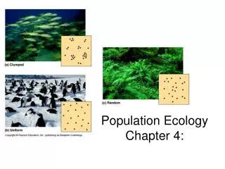
Dispersal patterns • 3 general patterns • Know these!!
1. Clumped Pattern • Most common pattern • Results form patchy environmental conditions-food, nutrient availability. • Ex: Mushrooms under rotting log. • Groups enhance predation • Safety. May increase chances for survival. • Ex: • Schooling behavior • Flocks of birds • humans
2. Uniform Dispersion • Individuals are evenly spaced • Results from direct antagonistic interactions • Plants secrete chemicals-inhibit nearby germination & competition (alleopathy) • territoriality
3. Random Dispersion • Spacing varies unpredictably • Absence of strong attractions or repulsions between individuals. • RARE pattern in nature • Example: windblown seeds land randomly & germinate.
Demography • Study of vital statistics of a population & how they change over time. • Add • Lose • 2 most important features • Age structure-relative numbers of individuals of each age group in a population • Sex ratios
1. Life Tables • How long, on average, are individuals of a given age expected to live. • Age-specific summary of survival patterns. • Follow the fate of a cohort (indiv. Of same age) from birth to death.
Do males or females have a higher death rate? Who lives longer?
2. Survivorship Curves • Graphic representation of data in Life Tables. • Plot of the proportion or numbers in a cohort still alive at each age. • 3 general Curve Types: ( be able to recognize and describe traits; members exhibiting each; example organism) • Type I—humans, elephants • Type II-squirrel • Type III-oysters, clam
Type I • Low early deaths. • Steep decline in death rates among those older • Produce few offspring, but provide good care. • Ex: • Humans • Other large mammals
Type II • Intermediate • Constant death rate over life span. • Ex: • Annual plants • small mammals ( grey squirrel), lizards
Type III • High death rates for the young. • ( sharp dip in curve initially) • Few live to adulthood • Associated with: • Produce large numbers of offspring-but provide little or no care. Ex: Oysters
Variations • Curve type may change between young and adults. • Ex: Nestlings - Type III Adult Birds- Type II • Stair-step curve • Invertebrates—crabs; high mortality during molt, followed by low mortality
Life-History Traits • Life History: Timing of reproduction and death. • Highly diverse, but do show patterns • Determines how populations grow. • Results from Natural Selection. • Darwinian “fitness”
Darwinian “fitness” • Survive AND Reproduce
Reproduction and survival—Life History Traits • 1. # of reproductive episodes • # offspring per reproductive episode • Age at first reproduction
2 Common Reproductive Patterns • 1. Semelparity: “big-bang” reproduction • 1 reproduction event • Salmon, agave ( desert plants) , annual plants • 2. Iteroparity • Fewer offspring at a time • Over many reproductive seasons
Population Studies & Reproductive Rates • Focusing on females and female offspring. • 2 Kinds of Reproductive Strategies identified • R • K
Life History Selection 1. "r" Selected species 2. "k" Selected species
“r" – Selected Species (density independent selection) • Increase fitness by producing as many offspring as possible. • Do this by one of these strategies: • Early maturation • Many reproductive events • Many offspring in one reproductive event • “Big bang” reproduction (semelparity) (pink salmon, agaves) is one time reproduction.
r-Selected Result • Maximize reproduction so that at least a few offspring survive to the next generation. • Most offspring die (Type III curve).
“K" – Selected Species (density dependent selection) • Increase fitness by having most offspring survive. • Maintain populations at or near “K” • Do this by: • High parental care • Late maturation • Few reproduction events • Few offspring.
K- Selected –Results.. • Maximize survivorship of each offspring . • Few offspring, but most survive (Type I curve).
What is the strategy • For a weed? • For Garden Pests?
POULATION GOWTH Zero population growth: Per capita birth + Per capita death=0
Exponential Growth • Produces a “J-shaped” growth curve. • Ideal conditions • unlimited resources. • Example: • Introduce into new or unfilled environment • Rebounding population
Population growth related to Life History Traits • S-shaped” growth curve. • Characteristic of “k" species. • Common when resources are limited.
Populations are limited by space, food. That limit is called the CARRYING CAPACITY • The graph shows a logistic population curve. • At what level do the deer reach their CARRYING CAPACITY?
What Limits Population Size? • Density-dependent factors: limited resources- space, food, water, air • related to population size • Density-independent factors: random occurrences that can limit population - earthquake, bad weather. • not affected by population size • Is disease density dependent, or density independent?
Additional Comments • Populations often overshoot “K” ( go beyond) , then drop back to or below “K”.
Regular Population Cycles • Cyclic changes in N over time. • Often seen in predator/prey cycles. • Ex: “Boom & Bust Cycle” of Snowshoe Hare -& Lynx
Predators kill and consume other organisms. Carnivores prey on animals, herbivores consume plants. • Predators usually limit the prey population, although in extreme cases they can drive the prey to extinction. • Why predators rarely kill and eat all the prey: • 1.Prey species often evolve protective mechanisms such as camouflage, poisons, spines, or large size to deter predation. • 2.Prey species often have refuges where the predators cannot reach them. • 3.Switch its prey as the prey species becomes lower in abundance:
Know how to read a graph for population growth, where K is; where the overshoot “K” is
Age Structure Diagrams • Show the percent of a population in different age categories . • Method to get data similar to a Life Table, but at one point in time.