Download
1 / 24
240 likes | 356 Views
FUR XII 2006 at LUISS in Roma . A METHODOLOGY FOR QUALITATIVE MODELLING OF ECONOMIC, FINANCIAL SYSTEMS WITH EMPHASIS TO CHAOS THEORY. Tom as V i cha , Mirko Dohnal Faculty of Business and Management, Brno University of Technology, Czech Republic vicha@fbm.vutbr.cz.

E N D
FUR XII 2006 at LUISS in Roma A METHODOLOGY FOR QUALITATIVE MODELLING OF ECONOMIC, FINANCIAL SYSTEMS WITH EMPHASIS TO CHAOS THEORY Tomas Vicha, Mirko Dohnal Faculty of Business and Management, Brno University of Technology, Czech Republic vicha@fbm.vutbr.cz
Introduction to Common Sense • The classical quantitative (i.e. analytical or statistical) analysis is not appropriate for some ill-known, difficult to measure, very complex and vague engineering problems • Low information intensity of the qualitative models offers the highest chance of success in development of a realistic i.e. applicable model. • Very often we need information such as variables will be rise or not – trend analysis. • Common-sense models (naive physics, qualitative model) offer a very flexible formal tool to deal with realistic engineering tasks.
Qualitative Modelling of Chaos • Identification of all possible chaotic behaviours which are qualitatively different can be done by brute force. • It means that all possible combinations of numerical values of all constants used in a model must be studied. • Qualitative models can identify not only all qualitative behaviours, but all possible transitions among them. • Complete sets of qualitative behaviours can, to certain level, characterize traditional quantitative phase portraits (more precisely state/scenario graph).
Qualitative Algebra – Intro 1. • A Qualitative value is + … increasing ,positive (k+) 0 … constant, zero (k0) - … decreasing, negative (k-) • A qualitative solution is specified if all its n qualitative variables: x1, x2, ..., xn are described in qualitative triplets: (X1, DX1, DDX1), (X2, DX2, DDX2), … (Xn, DXn, DDXn), whereXi is the i-th variable and DXi and DDXi are the first qualitative and second qualitative time derivations • A qualitative model has m qualitative solutions. The j-th qualitative state is the n-triplet: • (X1, DX1, DDX1), (X2, DX2, DDX2),… (Xn, DXn, DDXn)j, wherej =1, 2, …, m.
Qualitative Algebra – Intro 2. Qualitative addiction Qualitative multiplication Xi + Xj = Xs DXi + DXj = DXs DDXi + DDXj = DDXs Xi * Xj = Xs Xi * DXi + Xj * DXj = DXs
Methodology • Selection of a real-word model • Transformation of quantitative equations to qualitative equations • Assignment of follow up conditions • Transformation of qualitative equations to instruction set of a mathematical program – e.g. Q-SENECA • Definition of triplets of a qualitative variable • Make output questions • Computation of scenarios and transitions • Interpretation of result
M. 1) Selection of model • Damped Oscillation • Undamped Oscillation m … mass on a spring k … spring constant -bv … damping force x … position v … velocity (dx/dt) a … acceleration (dv/dt)
M. 2) Transform. to Qualitative Eq. • Ignore multiplicative quantitative constants • Additive constants can be solved by adding a new qualitative variable Damped Oscillation DDX + DX + X = 0 Undamped Oscillation DDX + X = 0
M. 3) Follow up Conditions • A relation between variables of a model is known. Thereafter complexity of the model can be reduced by assignment a follow up condition between variables. • It is not important for these models. If necessary, we could describe a relation of variables by the instruction set of Q-SENECA. • For example if two variables have linear relationship than we can use instruction: 1 23 VAR1 VAR2 0
M. 4) Transform. to Instruction Set • Note; 0 is a quantitative constant and that is why we have to replace it with an auxiliary variable ZERO. • Operations addition (ADD) and multiplication (MUL) need two parameters. That’s why we need the auxiliary variable P1 for the addition of DDX + DX + X. Damped Oscillation 1 d/t PX DPX 0 2 d/t DPX DDPX 0 3 ADD DDX DX P1 4 ADD P1 X ZERO Undamped Oscillation 1 d/t X DX 0 2 d/t DX DDX 0 3 ADD DDX X ZERO
M. 5) Definition of Triplets • We can restrict values of triplet (X, DX, DDX) or forbid computation of values of triplet (X, DX, DDX). The value of triplet is presented by the symbols from the set {+, -, 0, X (=count), * (=don’t count)}. DOTAZ ZERO 000 X XXX • The program will count with value of variable X and its first and second derivation … whole triplet of X
M. 6) Make Output Questions • We should set which variable(s) is(are) necessary for output. • For damped oscillation we need to compute outputs for X and DX. # X DX
M. 7) Computation of Scenarios Damped Oscillation DDX + DX + X = 0 Undamped Oscillation DDX + X = 0
M. 7) Computation of Transitions • Information as: from: scenario no. to: scenario no. Damped Undamped
M. 8) Interpretation of Result • The interpretation depends on the purpose of our modelling. • For example undamped oscillation has 9 scenarios. 8 are accessible and 1 is only for an extreme situation (no input energy – no oscillation, isolated scenario). All of 8 scenarios can be starting or terminating state/scenario. For each scenario is only one successor. • In this point it is good to compare qualitative results with quantitative system, see picture on the next slide. • Note: qualitative values of variable X / position (or DX / velocity) are described above (or under) time axis.
Predator Prey – Lotka Volterra • Predator prey – Lotka Voltera model (PPLV) is one of the oldest known chaotic models and was first used in theoretical biology by Lotka (1925) and Volterra (1931) • The basic non-linear differential equations concerning this mathematical approach are • where x is the prey, y the predator, α,β,γ and δ are all positive constants and the prime (') refers to x and y time derivatives.
PPLV Phase Space Picture 1) model A, B parameters: α=1, β=1, γ=1, δ=1 1) Time space portrait Phase space portrait 2) model C, D parameters: α=1, β=0.2, γ=1, δ=0.5 2)
PPLV – Economic Using • Where K is the prey or productive capacity or fixed capital stock and GDP the predator or gross domestic product (GDP) or simply production (by Kumimura). • An approach to the economical equilibrium theory has also been applied by Goodwin to another different context, that is, the employment capacity being the prey and employees salary being the predator.
PPLV Qualitative Analysis • The equations can be qualitatively rewritten as: DX + X*Y = X DY + Y = X*Y • PPLV qualitative computation is made for two settings: general setting (XXX) and positive settings of variables X, Y (+XX, see methodology chapter). The results are shown in the table. Model II. is illustrated by the graph of transitions, see next page.
Source Codefor Q-Seneca 1 d/t X DX 0 2 d/t Y DY 0 3 MUL XYP1 4 ADD DXP1X 5 ADD DYYP1 DOTAZ X +XX Y +XX # X Y Qualitative equations of PPLV: DX + X*Y = X DY + Y = X*Y
Conclusion • A result analysis is set of scenarios showing us general rules about a model. Moreover, set of qualitative scenarios and consequently qualitative transitions is a super set of existing solutions, because of potential spurious solutions. • The qualitative forecasting itself is very flexible. • Possible to perform any union or intersection of different models. Useful feature for verification of models and their simplification. This aspect is important for development of classical quantitative prediction models. • The classical statistical approach to model development is always based on a (semi) subjective choice of approximation curves. • The total number of qualitative scenarios is usually high. Multidimensional problems can have more than 10 000 scenarios.
Thank you for your attention A METHODOLOGY FOR QUALITATIVE MODELLING OF ECONOMIC, FINANCIAL SYSTEMS WITH EMPHASIS TO CHAOS THEORY Tomas Vicha, Mirko Dohnal Faculty of Business and Management, Brno University of Technology, Czech Republic vicha@fbm.vutbr.cz