Download
1 / 39
390 likes | 525 Views
On Threshold ARCH Models with Gram-Charlier Density. Xuan Zhou and W. K. Li Department of Statistics and Actuarial Science,HKU. Outline. Introduction to Threshold Model Introduction to Gram Charlier Density Threshold Model with Gram Charlier density Estimation method Testing method

E N D
On Threshold ARCH Models with Gram-Charlier Density Xuan Zhou and W. K. Li Department of Statistics and Actuarial Science,HKU
Outline • Introduction to Threshold Model • Introduction to Gram Charlier Density • Threshold Model with Gram Charlier density • Estimation method • Testing method • Empirical Results
Motivation • Some financial time series are asymmetric. • Investors are more nervous when the market is falling than when it is rising. Negative shocks entering the market lead to a larger return volatility than positive shocks of a similar magnitude. • Many models have been proposed to investigate this asymmetric feature, such as the ARCH-M model by Engle (1987) and the EGARCH model by Nelson (1990). • Innovation are believed to be non-Gaussian
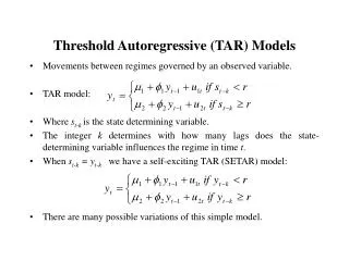
Threshold AR Model • Tong’s (1978) threshold autoregressive model • is the delay parameter, r is the threshold value.
Threshold ARCH Model • Li and Lam (1995) Threshold ARCH model
Conditional density • It is generally accepted that the conditional distribution of the asset return is not Gaussian (Mills(1995)). • The leptokurtosis has been found in most financial time series.
Introduction to Gram-Charlier (GC) density • The Gram-Charlier density is is the standard normal density function, and
Properties of GC density • The mean and variance are • The skewness and excess the kurtosis are and . • We use GC(u,h,s,k) to denote a GC density with mean u, variance h, skewness s, and excess kurtosis k.
Why Gram-Charlier density? • It nests Gaussian density. • It has explicit skewness and kurtosis.
Threshold ARCH Model with Gram Charlier Density is the indicator of regimes. Skewness and excess kurtosis will vary with time. The structure if different in different regimes.
Double Threshold ARCH model with GC density (DTARCHSK) is the indicator function
Estimation • Several problems in the estimation. • The number of parameters is large. • As pointed out by Bond (2001), MLE estimation is quite sensitive to initial parameters, therefore it'snecessary to search over a wide set of initial parameters beforeselecting the model with the highest likelihood value.
Estimation method: ECM • Step 1: For a given value of the skewness and kurtosis, fit the model by MLE. • Step 2: Conditional on the estimates, calculate the residuals. Find the maximum likehood estimates of the skewness and the kurtosis of the residuals. • Step 3: Repeat until all the parameters converge. Group one Group two
The convergence is fast. Almost every simulation converges in three iterations. • The first step of the ECM method is a quasi-maximum likelihood estimation. It converges when the third and fourth moments are assumed finite. Therefore, the assumed value for the skewness and kurtosis would not affect Step 1 much. The parameters for mean and variance structure converge fast. All estimates converged within three iterations.
Lagrange Multiplier Test • The threshold structure and GC density both can help explain the asymmetric features, combination of them will definitely enhance the model's ability to capture asymmetry. • On the other hand, they will also interact with each other and prevent us to distinguish them.
Example • Consider the model • When the previous data is positive, the conditional density is skewed to the positive side. When the previous data is negative, the conditional density is still skewed to the positive side. Therefore, the behavior of the series is asymmetric even the mean structure is symmetric.
Wong and Li’s (1997) test does not take into account the conditional density. Their nominal 5% test on the model reject 8% of the experiments.
Lagrange Multiplier test • The null hypothesis is: • The conditional likelihood function is:
Lagrange Multiplier test • The fish information matrix is • Score function is
Because the conditional density is symmetric, we can show that (Engle’s (1982) theorem), The information matrix is block diagonal. Therefore, we can drop the second block of the matrix which is not related to the threshold structure in the test.
As the time series is stationary and ergodic, by the martingale central limit theorem, we can show
Supreme Lagrange Multiplier Test • If r is given, define the Lagrange-Multiplier test statistic as • If r is unknown, we define the supreme Lagrange-Multiplier test statistic as • The distribution of S was proved to berelated to an Ornstein-Uhlenbeck (O-U) process (Chan(1990)).
Effect of the skewness in the testing • When the skewness is included in the GC density, the information matrix is no longera block diagonal matrix. Therefore we can not just drop the secondblock of the matrix. As a result, the form of the Lagrange Multiplier test will be morecomplicated to handle. • However, the critical value of the testfor the models with skewed density are almost the same as the test of thecorresponding models with non-skewed density.
Empirical results • We apply our model to several foreign exchange rates series,including British Pound (GBP/USD), Japanese Yen/USD (JPY/USD),German Mark (GEM/USD) from Jan 2, 1990 to Dec 29, 2000. • Fit the data with four models: ARCH, ARCHSK, DTARCH and DTARCHSK model.
Test results • The test of DTARCHSK and the test of DTARCH generate very differentconclusions on the existence of threshold structure. The test ofDTARCH is more likely to reject the null hypothesis while theproposed one prefers the null hypothesis. This is because the ARCHSKmodel has captured most of the asymmetric features and need not tofurther assign threshold structure.
Some Conditional density Model • Engle and Gonzalez- Rivera (1991) Semiparametric ARCH models. • Harvey and Siddique (1999) Autoregressive conditional skewness • Brooks et al.(2005) Autoregressive conditional kurtosis • The skewness and the kurtosis of Student’s t-density have to be calculated from the distributional parameters. How skewed and howleptokurtic the density is can not be conveyed directly.