Download
1 / 38
400 likes | 689 Views
Geometric Models & Camera Calibration. Reading: Chap. 2 & 3. Introduction. We have seen that a camera captures both geometric and photometric information of a 3D scene. Geometric: shape, e.g. lines, angles, curves Photometric: color, intensity

E N D
Geometric Models & Camera Calibration Reading: Chap. 2 & 3
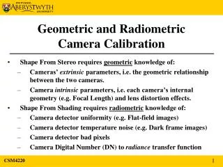
Introduction • We have seen that a camera captures both geometric and photometric information of a 3D scene. • Geometric: shape, e.g. lines, angles, curves • Photometric: color, intensity • What is the geometric and photometric relationship between a 3D scene and its 2D image? • We will understand these in terms of models.
Models • Models are approximations of reality. • “Reality” is often too complex, or computationally intractable, to handle. • Examples: • Newton’s Laws of Motion vs. Einstein’s Theory of Relativity • Light: waves or particles? • No model is perfect. • Need to understand its strengths & limitations.
least accurate most accurate Camera Projection Models • 3D scenes project to 2D images • Most common model: pinhole camera model • From this we may derive several types of projections: • orthographic • weak-perspective • para-perspective • perspective
Pinhole Camera Model real image plane virtual image plane optical centre object Z Y f f image is inverted image is not inverted
Real vs. Virtual Image Plane • The image is physically formed on the real image plane (retina). • The image is vertically and laterally inverted. • We can imagine a virtual image plane at a distance of f in front of the camera optical center, where f is the focal length. • The image on this virtual image plane is not inverted. • This is actually more convenient. • Henceforth, when we say “image plane” we will mean the virtual image plane.
Perspective Projection • The imaging process is a many-to-one mapping • all points on the 3D ray map to a single image point. • Therefore, depth information is lost • From similar triangles, can write down the perspective equation:
Perspective Projection This assumes coordinate axes is at the pinhole.
3D Scene point P Camera coordinate system Rotation R t: World origin w.r.t. camera coordinate axes World coordinate system P : 3D position of scene point w.r.t world coordinate axes R : Rotation matrix to align world coordinate axes to camera axes
PerspectiveProjection α, β : scaling in image u, v axes, respectively Θ : skew angle, that is, angle between u, v axes u0, v0 : origin offset Note: α=kf, β=lf where k, l are the magnification factors
Intrinsic vs. Extrinsic parameters • Intrinsic: internal camera parameters. • 6 of them (5 if you don’t care about focal length) • Focal length, horiz. & vert. magnification, horiz. & vert. offset, skew angle • Extrinsic: external parameters • 6 of them • 3 rotation angles, 3 translation param • Imposing assumptions will reduce # params. • Estimating params is called camera calibration.
Z Y X Representing Rotations • Euler angles • pitch: rotation about x axis : • yaw: rotation about y axis: • roll: rotation about z axis:
Rotation Matrix Two properties of rotation matrix: R is orthogonal: RTR = I det(R) = 1
Parallel lines optical axis Camera centre Orthographic Projection Projection rays are parallel Image plane
Orthographic Projection Equations : first two rows of R : first two elements of t This projection has 5 degrees of freedom.
Parallel lines Image plane Weak-perspective Projection
Weak-perspective Projection This projection has 7 degrees of freedom.
Parallel lines Image plane Para-perspective Projection
Para-perspective Projection • Camera matrix given in textbook Table 2.1, page 36. • Note: Written a bit differently. • This has 9 d.o.f.
Real cameras • Real cameras use lenses • Lens distortion causes distortion in image • Lines may project into curves • See Chap 1.2, 3.3 for details • Change of focal length (zooming) scales the image • not true if assuming orthographic projection) • Color distortions too
Color Aberration • Bad White Balance
Color Aberration • Purple Fringing
Color Aberration • Vignetting
Recap • A general projective matrix: • This has 11 d.o.f. , i.e. 11 parameters • 5 intrinsic, 6 extrinsic • How to estimate all of these? • Geometric camera calibration
Key Idea • Capture image of a known 3D object (calibration object). • Establish correspondences between 3D points and their 2D image projections. • Estimate M • Estimate K, R, and t from M • Estimation can be done using linear or non-linear methods. • We will study linear methods first.
Setting things up • Calibration object: • 3D object, or • 2D planar object captured at different locations
Setting it up • Suppose we have N point correspondences: • P1, P2, … PN are 3D scene points • u1, u2, … uN are corresponding image points • Let mT1, mT2, mT3 be the 3 rows of M • Let (ui, vi) be the (non-homogeneous) coords of the i th image point. • Let Pi be the homogeneous coords of i th scene point.
Math • For the i th point • Each point gives 2 equations. • Using all N points gives 2N equations:
Math A m = 0 A : 2N x 12 matrix, rank is 11 m : 12 x 1 column vector Note that m has only 11 d.o.f.
Math • Solution? • m is in the Nullspace of A ! • Use SVD: A = U ∑ VT • m = last column of V • m is only up to an unknown scale • In this case, SVD solution makes || m || = 1
Estimating K, R, t • Now that we have M (3x4 matrix) • c is the 3D coords of camera center wrt World axes • Let ĉ be homogeneous coords of c • It can be shown that M ĉ = 0 • So ĉ is in the Nullspace of M • And t is computed from –Rc, once R is known.
Estimating K, R, t • B, the left 3x3 submatrix of M is KR • Perform “RQ” decomposition on B. • The “Q” is the required rotation matrix R • And the upper triangular “R” is our K matrix ! • Impose the condition that diagonals of K are positive • We are done!
RQ factorization • Any n x n matrix A can be factored into A = RQ • Where both R, Q are n x n • R is upper triangular, Q is orthogonal • Not the same as QR factorization • Trick: post multiply A by Givens rotation matrices: Qx ,Qy, Qz
RQ factorization • c, s chosen to make a particular entry of A zero • For example, to make a21 = 0, we solve • Choose Qx ,Qy, Qz such that
Degeneracy • Caution: The 3D scene points should not all lie on a plane. • Otherwise no solution • In practice, choose N >= 6 points in “general position” • Note: the above assumes no lens distortion. • See Chap 3.3 for how to deal with lens distortion.
Summary • Presented pinhole camera model • From this we get hierarchy of projection types • Perspective, Para-perspective, Weak-perspective, Orthographic • Showed how to calibrate camera to estimate intrinsic + extrinsic parameters.