Download

1 / 19
200 likes | 423 Views
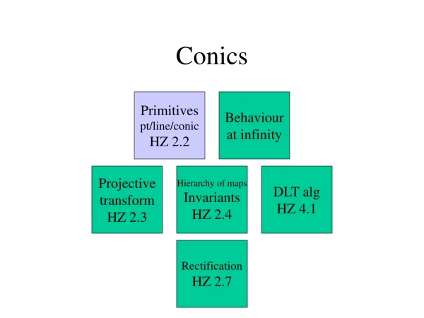
Conics. Primitives pt/line/conic HZ 2.2. Behaviour at infinity. Projective transform HZ 2.3. Hierarchy of maps Invariants HZ 2.4. DLT alg HZ 4.1. Rectification HZ 2.7. Conic representation. conic = plane curve described by quadratic polynomial = section of cone

E N D
Conics Primitives pt/line/conic HZ 2.2 Behaviour at infinity Projective transform HZ 2.3 Hierarchy of maps Invariants HZ 2.4 DLT alg HZ 4.1 Rectification HZ 2.7
Conic representation • conic = plane curve described by quadratic polynomial = section of cone • what are the conics? • important primitives for vision and graphics • conic in Euclidean space: ax^2 + bxy + cy^2 + dx + ey + f = 0 • homogenize to translate to projective space • 2-minute exercise: how do you homogenize this polynomial and thereby translate to projective space? • conic in projective space: ax^2 + bxy + cy^2 + dxw + eyw + fw^2 = 0 • observation: homogenize a polynomial by the replacement x x/w and y y/w (ring a bell?) • this conic in projective space is encoded by a symmetric 3x3 matrix: • x^t C x =0 • C = [a, b/2, d/2; b/2, c, e/2; d/2, e/2, f] • ijth entry encodes ijth coefficient (where x=1,y=2,w=3) • 2-minute exercise: how many degrees of freedom does a conic have?
Conic representation 2 • matrix C is projective (only defined up to a multiple) • conic has 5dof: ratios {a:b:c:d:e:f} or 6 matrix entries of C minus scale • kC represents the same conic as C (equivalent to multiplying equation by a constant) • in P^2, all conics are equivalent • that is, can transform from a conic to any other conic using projective transforms • not true in Euclidean space: cannot transform from ellipse to parabola using linear transformation • transformation rule: • if point x Hx, then conic C (H-1)^t C H-1 • HZ30-31, 37
Conic tangents • another calculation is made simple in projective space (and reduces to matrix computation) • Result: The tangent of the conic C at the point x is Cx. • Proof: • this line passes through x since x^t Cx = 0 (x lies on the conic) • Cx does not contain any other point y of C, otherwise the entire line between x and y would lie on the conic: • if y^t C y = 0 (y lies on conic) and x^t C y = 0 (Cx contains y), then x+\alpha y (the entire line between x and y) also lies on C • thus, Cx is the tangent through x (a tangent is a line with only one point of contact with conic) • HZ31
Metric rectification with circular points Primitives pt/line/conic HZ 2.2 Behaviour at infinity Projective transform HZ 2.3 Hierarchy of maps Invariants HZ 2.4 DLT alg HZ 4.1 Rectification HZ 2.7
Material for metric rectification • circular points (34) • similarity iff fixed circular points (52) • conic (55) • dual conic • degenerate conic • C*∞: conic dual to circular points (or just dual conic) • angle from dual conic • image of dual conic under homography • then we’re ready for the algorithm of Example 2.26 HZ
Line conic • we have considered point conic • points are dual to lines: let’s dualize • suppose conic is nondegenerate (not 2 lines or repeated line), so C is nonsingular • 3x3 matrix C encodes the points of a conic • x^t C x = 0 if x lies on conic • matrix C-1 encodes the tangent lines of that conic: • L is a tangent line of the conic iff • L^t C-1 L = 0 • proof: tangent L = Cx for some point x on conic; x^t C x = 0 so substituting x = C-1L yields (C-1L)^t C (C-1L) = L^t C-1L = 0 (recall that C is symmetric) • called a dual conic or line conic; conic envelope • transformation rule: if point x Hx, then dual conic C* H C* H^t • HZ31,37
Degenerate conics • there are degenerate point conics and degenerate line conics • recall the outer product • if L and M are lines, LM^t + ML^t is the degenerate point conic consisting of these two lines • notice that the matrix is singular (rank 2) • if p and q are points, pq^t + qp^t is the degenerate line conic consisting of all lines through p or q • [2 pencils of lines, drawing] • notice that this is a line conic (or dual conic)
‘The’ dual conic C*∞ • two circular points I and J • make a degenerate line conic out of them • C*∞ = IJ^t + JI^t = (1,0,0; 0,1,0; 0,0,0) • all lines through the circular points • C*∞ will be called ‘the’ dual conic • although it is the line conic dual to the circular points • like circular points, C*∞ is fixed under a projective transform iff it is a similarity • interesting fact: null vector of C*∞ = line at infinity • HZ 52-54 • explore relationship to angle
Computing angle from C*∞ • how can we measure angle in a photograph? • angle is typically measured using dot product • but dot product is not invariant under homography • consider two lines L and M in projective space (viewed as conventional columns, not correct rows) • L^t M is replaced by a normalized L^t C*∞ M • (L^t C*∞ M) / \sqrt( (L^t C*∞ L) (M^t C*∞ M)) • this is invariant to homography • note that L^t C*∞ M is equivalent to dot product in the original space • (a1,a2,1) C*∞ (b1,b2,1) = a1b1 + a2b2 • Result: (L^t C*∞ M) / \sqrt( (L^t C*∞ L) (M^t C*∞ M)) is the appropriate measure of angle in projective space. • since angle = arccos (A.B), this is of course a measure of cos(angle), not angle • corollary: angle can be measured once C*∞ is known • HZ54-55
How C*∞ transforms • we want to understand how C*∞ transforms under a homography (since we don’t want it to transform!) • a homography matrix can be decomposed into a projective, affine, and similarity component: • H = [I 0] [K 0] [sR t] [v^t 1] [0 1] [0 1] = Hp Ha Hs • note that K is the affine component • recall that line conics transform by C* H C* H^t, so • C*∞ (Hp Ha Hs) C*∞ (Hp Ha Hs)t • but the dual conic is fixed under a similarity, so: • C*∞ (Hp Ha) C*∞ (Hp Ha)t • which reduces as follows using C*∞ = diag(1,1,0): • image of C*∞= [KK^t KK^t v ] • [v^t KK^t v^t KK^t v ] • when line at infinity is not moving, v = 0: • image of C*∞ in an affinely rectified image = [KK^t 0] [0 0] • [HZ43 for this decomposition chain of a homography, HZ55]
Metric rectification algorithm • “We have the technology. We can rebuild him!” • input: 2 orthogonal line pairs • assume that the image has already been affinely rectified (i.e., line at infinity is in correct position) • we are within an affinity of a similarity! • what is this affinity K? use the known orthogonality (known angle) to solve for K • let S = KK^t: we actually solve for S, then retrieve K using Cholesky decomposition • note: S has 2 dof (symmetric 2x2) • use the two line angle constraints to solve for these dof
Metric rectification continued • (L,M) = image of orthogonal line pair • Figure 2.17a • choose two points P1,P2 on L: L = P1xP2 • L = (L1,L2,L3) and M = (M1,M2,M3) • orthogonal pair (L,M) satisfies Lt C*∞ M = 0 • Lt [S 0; 0 0] M = (L1 L2) S (M1 M2) • this imposes a linear constraint on S • (L1 M1, L1M2 + L2M1, L2M2) . (s11, s12, s22) = 0 • first row of matrix . S = 0 • a second orthogonal pair defines the 2nd row of the system As = 0 [A for angle] • A is 2x3 matrix, s is the vector (s11,s12,s22) • S is the null vector of this matrix M • Cholesky decompose S to retrieve K • the ‘true’ image (up to metric structure) must have been mapped by the affinity [K 0; 0,1] • see ‘how C*∞ transforms’ above • so rectify by mapping image by K-1 • Moral: use orthogonal constraint to solve for affinity K, using the dual conic to help you measure angle • note: never actually compute dual conic, just rely on its properties • this is a perfect example of the power of a theoretical construct • HZ56
Synopsis • want affinity K • want S = KK^t • S is available from the image of C*∞ • get at image of C*∞ using angle relationship • use orthogonal pairs to solve for image of C*∞ • back out from image of C*∞ to S to K
Numerical aside: solving for null space • to solve Ax = 0: • compute SVD of A = U D V^t • if null space is 1d, x = last column of V (called null vector) • in general, last d columns of V span the d-dimensional null space
Numerical aside: SVD • singular value decomposition of A is A = U D V^t, where • mxn A • mxm orthogonal U • mxn diagonal D (containing singular values sorted) • nxn orthogonal V • do not compute yourself! • compute using CLAPACK or OpenCV
Other methods for metric rectification • the 2-ortho-pair method is called stratified rectification • stratification = 2 step approach to removal of distortion, first projective, then affine • Note: 2 orthogonal lines are conjugate with respect to the dual conic C*∞ • can also rectify (in a stratified fashion) using an imaged circle • image of circle is ellipse: intersect it with vanishing line to find imaged circular points • can also rectify using 5 orthogonal line pairs • why would you want to? because it doesn’t assume image has already been affinely rectified • method (your responsibility to read) • find the dual conic as the null vector of a 5x6 matrix built up from 5 linear equations • see DLT algorithm below for a similar approach (this is a very popular approach!) • note: solving for entire 5dof conic, not just the 2dof affine component • HZ56-57
On OpenCV • review openCVInstallationNotes • OpenCV demo programs at my website • cvdemo, cvmousedemo, cvresizedemo, cvpixeldemo • opencvlibrary.sourceforge.net • invaluable resource for full documentation, FAQ, examples, Wiki • IPL = Image Processing Library • depth = # of bits in each data value of image • 8 = uchar, 32 = float • channels = # of data values for each image pixel • 1 = grayscale; 3 = RGB
Capturing images as test data • I would like you to personalize your test data • I would also like to gather an image database • assignment: find images replete with parallel lines (and optimally, vanishing lines inside the image) and orthogonal lines • also want different directions of parallel and orthogonal lines: e.g., brick wall is not as useful since all parallel lines yield only two distinct ideal points • challenge: rectification without gaps • challenge: rectification to within a translation using external cues • challenge: rectification from other constraints (e.g., in a natural scene with no visible lines or circles) • challenge: image contexts with circles and other known nonlinear curves