Download
1 / 29
290 likes | 483 Views
Confidence intervals and hypothesis testing. Petter Mostad 2005.10.03. Confidence intervals (repetition). Assume μ and σ 2 are some real numbers, and assume the data X 1 ,X 2 ,…,X n are a random sample from N( μ , σ 2 ). Then thus so

E N D
Confidence intervals and hypothesis testing Petter Mostad 2005.10.03
Confidence intervals (repetition) • Assume μ and σ2 are some real numbers, and assume the data X1,X2,…,Xnare a random sample from N(μ,σ2). • Then • thus • so and we say that is a confidence interval for μ with 95% confidence, based on the statistic
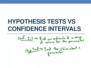
Confidence intervals, general idea • We have a model with an unknown parameter • We find a ”statistic” (function of the sample) with a known distribution, depending only on the unknown parameter • This distribution is used to construct an interval with the following property: If you repeat many times selecting a parameter and simulating the statistic, then about (say) 95% of the time, the confidence interval will contain the parameter
Hypothesis testing • Selecting the most plausible model for the data, among those suggested • Example: Assume X1,X2,…,Xnis a random sample from N(μ,σ2), where σ2is known, but μis not; we want to select μfitting the data. • One possibility is to look at the probability of observing the data given different values for μ. (We will return to this) • Another is to do a hypothesis test
Example • We select two alternative hypotheses: • H0: • H1: • Use the value of to test H0 versus H1: If is far from , it will indicate H1. • Under H0, we know that • Reject H0 if is outside
General outline for hypothesis testing • The possible hypotheses are divided into H0, the null hypothesis, and H1, the alternative hypothesis • A hypothesis can be • Simple, so that it is possible to compute the probability of data (e.g., ) • Composite, i.e., a collection of simple hypotheses (e.g., )
General outline (cont.) • A test statistic is selected. It must: • Have a higher probability for ”extreme” values under H1 than under H0 • Have a known distribution under H0 (when simple) • If the value of the test statistic is ”too extreme”, then H0 is rejected. • The probability, under H0, of observing the given data or something more extreme is called the p-value. Thus we reject H0 if the p-value is small. • The value at which we reject H0 is called the significance level.
Note: • There is an asymmetry between H0 and H1: In fact, if the data is inconclusive, we end up not rejecting H0. • If H0 is true the probability to reject H0 is (say) 5%. That DOES NOT MEAN we are 95% certain that H0 is true! • How much evidence we have for choosing H1 over H0 depends entirely on how much more probable rejection is if H1 is true.
Errors of types I and II • The above can be seen as a decision rule for H0 or H1. • For any such rule we can compute (if both H0 and H1 are simple hypotheses): 1 - power H0 true H1 true Accept H0 TYPE II error Reject H0 TYPE I error Significance
Significance and power • If H0 is composite, we compute the significance from the simple hypothesis that gives the largest probability of rejecting H0. • If H1 is composite, we compute a power value for each simple hypothesis. Thus we get a power function.
Example 1: Normal distribution with unknown variance • Assume • Then • Thus • So a confidence interval for , with significance is given by
Example 1 (Hypothesis testing) • Hypotheses: • Test statistic under H0 • Reject H0 if or if • Alternatively, the p-value for the test can be computed (if ) as the such that
Example 1 (cont.) • Hypotheses: • Test statistic assuming • Reject H0 if • Alternatively, the p-value for the test can be computed as the such that
Example 1 (cont.) • Assume that you want to analyze as above the data in some column of an SPSS table. • Use ”Analyze” => ”Compare means” => ”One-sample T Test” • You get as output a confidence interval, and a test as the one described above. • You may adjust the confidence level using ”Options…”
Example 2: Differences between means • Assume and • We would like to study the difference • Four different cases: • Matched pairs • Known population variances • Unknown but equal population variances • Unknown and possibly different pop. variances
Known population variances • We get • Confidence interval for
Unknown but equal population variances • We get where • Confidence interval for
Hypothesis testing: Unknown but equal population variances • Hypotheses: • Test statistic: • Reject H0 if or if ”T test with equal variances”
Unknown and possibly unequal population variances • We get where • Conf. interval for
Hypothesis test: Unknown and possibly unequal pop. variances • Hypotheses: • Test statistic • Reject H0 if or if ”T test with unequal variances”
Practical examples: • The lengths of children in a class are measured at age 8 and at age 10. Use the data to find an estimate, with confidence limits, on how much children grow between these ages. • You want to determine whether a costly operation is generally done more cheaply in France than in Norway. Your data is the actual costs of 10 such operations in Norway and 20 in France.
Example 3: Population proportions • Assume , so that is a frequency. • Then • Thus • Thus • Confidence interval for (approximately, for large n) (approximately, for large n)
Example 3 (Hypothesis testing) • Hypotheses: • Test statistic under H0, for large n • Reject H0 if or if
Example 4: Differences between population proportions • Assume and , so that and are frequencies • Then • Confidence interval for (approximately)
Example 4 (Hypothesis testing) • Hypotheses: • Test statistic where • Reject H0 if
Example 5: The variance of a normal distribution • Assume • Then • Thus • Confidence interval for
Example 6: Comparing variances for normal distributions • Assume • We get • Fnx-1,ny-1 is an F distribution with nx-1 and ny-1 degrees of freedom • We can use this exactly as before to obtain a confidence interval for and for testing for example if • Note: The assumption of normality is crucial!
Sample size computations • For a sample from a normal population with known variance, the size of the conficence interval for the mean depends only on the sample size. • So we can compute the necessary sample size to match a required accuracy • Note: If the variance is unknown, it must somehow be estimated on beforehand to do the computation • Works also for population proportion estimation, giving an inequality for the required sample size
Power computations • If you reject H0, you know very little about the evidence for H1 versus H0 unless you study the power of the test. • The power is 1 minus the probability of rejecting H0 given that a hypothesis in H1 is true. • Thus it is a function of the possible hypotheses in H1. • We would like our tests to have as high power as possible.