Download
1 / 55
680 likes | 978 Views
Maclaurin and Taylor Polynomials. Objective: Improve on the local linear approximation for higher order polynomials. Local Quadratic Approximations.

E N D
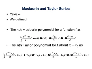
Maclaurin and Taylor Polynomials Objective: Improve on the local linear approximation for higher order polynomials.
Local Quadratic Approximations • Remember we defined the local linear approximation of a function f at x0 as . In this formula, the approximating function is a first-degree polynomial. The local linear approximation of f at x0 has the property that its value and the value of its first derivative match those of f at x0.
Local Quadratic Approximations • If the graph of a function f has a pronounced “bend” at x0 , then we can expect that the accuracy of the local linear approximation of f at x0 will decrease rapidly as we progress away from x.
Local Quadratic Approximations • One way to deal with this problem is to approximate the function f at x0 by a polynomial p of degree 2 with the property that the value of p and the values of its first two derivatives match those of f at x0. This ensures that the graphs of f and p not only have the same tangent line at x0 , but they also bend in the same direction at x0. As a result, we can expect that the graph of p will remain close to the graph of f over a larger interval around x0. The polynomial p is called the local quadratic approximation of f at x = x0.
Local Quadratic Approximations • We will try to find a formula for the local quadratic approximation for a function f at x = 0. This approximation has the form where c0 , c1 , and c2 must be chosen so that the values of and its first two derivatives match those of f at 0. Thus, we want
Local Quadratic Approximations • The values of p(0), p /(0), and p //(0) are as follows:
Local Quadratic Approximations • Thus it follows that • The local quadratic approximation becomes
Example 1 • Find the local linear and local quadratic approximations of ex at x = 0, and graph ex and the two approximations together.
Example 1 • Find the local linear and local quadratic approximations of ex at x = 0, and graph ex and the two approximations together. • f(x)= ex, so • The local linear approximation is • The local quadratic approximation is
Example 1 • Find the local linear and local quadratic approximations of ex at x = 0, and graph ex and the two approximations together. • Here is the graph of the three functions.
Maclaurin Polynomials • It is natural to ask whether one can improve the accuracy of a local quadratic approximation by using a polynomial of degree 3. Specifically, one might look for a polynomial of degree 3 with the property that its value and the values of its first three derivatives match those of f at a point; and if this provides an improvement in accuracy, why not go on to polynomials of higher degree?
Maclaurin Polynomials • We are led to consider the following problem:
Maclaurin Polynomials • We will begin by solving this problem in the case where x0 = 0. Thus, we want a polynomial • such that
Maclaurin Polynomials • But we know that
Maclaurin Polynomials • But we know that • Thus we need
Maclaurin Polynomials • This yields the following values for the coefficients of p(x)
Maclaurin Polynomials • This leads us to the following definition.
Example 2 • Find the Maclaurin Polynomials p0 , p1, p2 , p3, and pn for ex.
Example 2 • Find the Maclaurin Polynomials p0 , p1, p2 , p3, and pn for ex. • We know that • so
Example 2 • Why do I need to memorize this? • They may ask you to find a Maclaurin polynomial to approximate xex. This is what they want you to do:
Example 2 • Find the Maclaurin Polynomials p0 , p1, p2 , p3, and pn for ex. • The graphs of ex and all four approximations are shown.
Taylor Polynomials • Up to now we have focused on approximating a function f in the vicinity of x = 0. Now we will consider the more general case of approximating f in the vicinity of an arbitrary domain value x0.
Taylor Polynomials • Up to now we have focused on approximating a function f in the vicinity of x = 0. Now we will consider the more general case of approximating f in the vicinity of an arbitrary domain value x0. • The basic idea is the same as before; we want to find an nth-degree polynomial p with the property that its value and the values of its first n derivatives match those of f at x0. However, rather than expressing p(x) in powers of x, it will simplify the computation if we express it in powers of x – x0; that is
Taylor Polynomial • This leads to the following definition:
Example 3 • Find the first four Taylor Polynomials for lnx about x = 2.
Example 3 • Find the first four Taylor Polynomials for lnx about x = 2. • Let f(x) = lnx. Thus
Example 3 • Find the first four Taylor Polynomials for lnx about x = 2. • This leads us to:
Example 3 • Find the first four Taylor Polynomials for lnx about x = 2. • The graphs of all five polynomials are shown.
Sigma Notation • Frequently we will want to express a Taylor Polynomial in sigma notation. To do this, we use the notation f k(x0) to denote the kth derivative of f at x = xo , and we make the connection that f 0(x0) denotes f(x0). This enables us to write
Example 4 • Find the nth Maclaurin polynomials for (a) (b) (c)
Example 4 • Find the nth Maclaurin polynomials for (a) (b) (c) (a)
Example 4 • Find the nth Maclaurin polynomials for (a) (b) (c) (a) This leads us to:
Example 4 • Find the nth Maclaurin polynomials for (a) (b) (c) (a) This leads us to:
Example 4 • Find the nth Maclaurin polynomials for (a) (b) (c) (a) The graphs are shown.
Example 4 • Find the nth Maclaurin polynomials for (a) (b) (c) (b) We start with:
Example 4 • Find the nth Maclaurin polynomials for (a) (b) (c) (b) This leads us to:
Example 4 • Find the nth Maclaurin polynomials for (a) (b) (c) (b) This leads us to:
Example 4 • Find the nth Maclaurin polynomials for (a) (b) (c) (b) The graphs are shown.
Example 4 • Find the nth Maclaurin polynomials for (a) (b) (c) You need to memorize these!
Example 4 • Find the nth Maclaurin polynomials for (a) (b) (c) You need to memorize these!
Example 4 • Find the nth Maclaurin polynomials for (a) (b) (c) You need to memorize these!
Example 4 • Find the nth Maclaurin polynomials for (a) (b) (c) (c) We start with:
Example 4 • Find the nth Maclaurin polynomials for (a) (b) (c) (c) We start with:
Example 4 • Find the nth Maclaurin polynomials for (a) (b) (c) (c) This leads us to • You should memorize this as well.
The nth Remainder • It will be convenient to have a notation for the error in the approximation . Accordingly, we will let denote the difference between f(x) and its nth Taylor polynomial: that is • This can also be written as:
The nth Remainder • The function is called the nth remainder for the Taylor series of f, and the formula below is called Taylor’s formula with remainder.
The nth Remainder • Finding a bound for gives an indication of the accuracy of the approximation . The following theorem provides such a bound. • The bound, M, is called the Lagrange error bound.
Example 6 • Use an nth Maclaurin polynomial for to approximate e to five decimal places.
Example 6 • Use an nth Maclaurin polynomial for to approximate e to five decimal places. • The nth Maclaurin polynomial for is • from which we have
Example 6 • Use an nth Maclaurin polynomial for to approximate e to five decimal places. • Our problem is to determine how many terms to include in a Maclaurin polynomial for to achieve five decimal-place accuracy; that is, we want to choose n so that the absolute value of the nth remainder at x = 1 satisfies