Download
1 / 57
610 likes | 899 Views
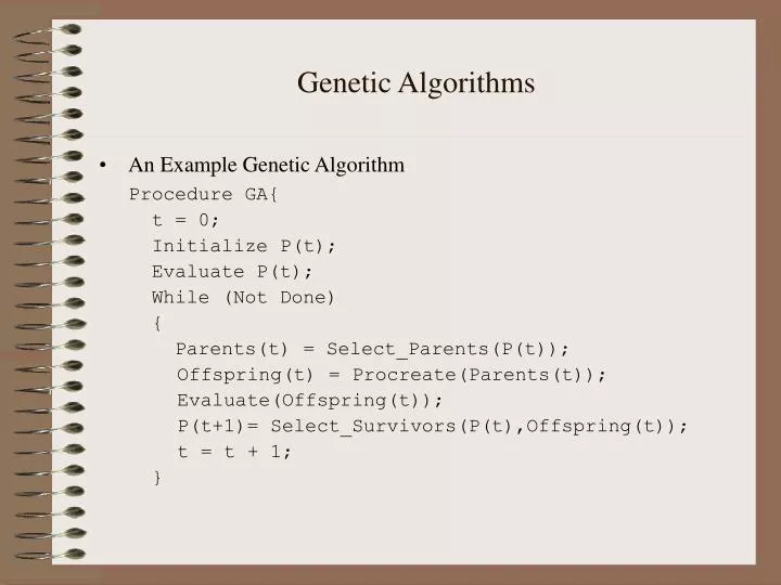
Genetic Algorithms. An Example Genetic Algorithm Procedure GA{ t = 0; Initialize P(t); Evaluate P(t); While (Not Done) { Parents(t) = Select_Parents(P(t)); Offspring(t) = Procreate(Parents(t)); Evaluate(Offspring(t));

E N D
Genetic Algorithms • An Example Genetic Algorithm Procedure GA{ t = 0; Initialize P(t); Evaluate P(t); While (Not Done) { Parents(t) = Select_Parents(P(t)); Offspring(t) = Procreate(Parents(t)); Evaluate(Offspring(t)); P(t+1)= Select_Survivors(P(t),Offspring(t)); t = t + 1; }
Genetic AlgorithmsRepresentation of Candidate Solutions • GAs on primarily two types of representations: • Binary-Coded • Real-Coded • Binary-Coded GAs must decode a chromosome into a CS, evaluate the CS and return the resulting fitness back to the binary-coded chromosome representing the evaluated CS.
Genetic Algorithms:Binary-Coded Representations • For Example, let’s say that we are trying to optimize the following function, • f(x) = x2 • for 2 x 1 • If we were to use binary-coded representations we would first need to develop a mapping function form our genotype representation (binary string) to our phenotype representation (our CS). This can be done using the following mapping function: • d(ub,lb,l,chrom) = (ub-lb) decode(chrom)/(2l-1) + lb
Genetic Algorithms:Binary-Coded Representations • d(ub,lb,l,c) = (ub-lb) decode(c)/(2l-1) + lb , where • ub = 2, • lb = 1, • l = the length of the chromosome in bits • c = the chromosome • The parameter, l, determines the accuracy (and resolution of our search). • What happens when l is increased (or decreased)?
Genetic Algorithms:Real-Coded Representations • Real-Coded GAs can be regarded as GAs that operate on the actual CS (phenotype). • For Real-Coded GAs, no genotype-to-phenotype mapping is needed.
Genetic Algorithms:Parent Selection Methods • An Example Genetic Algorithm Procedure GA{ t = 0; Initialize P(t); Evaluate P(t); While (Not Done) { Parents(t) = Select_Parents(P(t)); Offspring(t) = Procreate(Parents(t)); Evaluate(Offspring(t)); P(t+1)= Select_Survivors(P(t),Offspring(t)); t = t + 1; }
Genetic Algorithms:Parent Selection Methods • GA researchers have used a number of parent selection methods. Some of the more popular methods are: • Proportionate Selection • Linear Rank Selection • Tournament Selection
Genetic Algorithms:Proportionate Selection • In Proportionate Selection, individuals are assigned a probability of being selected based on their fitness: • pi = fi / fj • Where pi is the probability that individual i will be selected, • fi is the fitness of individual i, and • fj represents the sum of all the fitnesses of the individuals with the population. • This type of selection is similar to using a roulette wheel where the fitness of an individual is represented as proportionate slice of wheel. The wheel is then spun and the slice underneath the wheel when it stops determine which individual becomes a parent.
Genetic Algorithms:Proportionate Selection • There are a number of disadvantages associated with using proportionate selection: • Cannot be used on minimization problems, • Loss of selection pressure (search direction) as population converges, • Susceptible to Super Individuals
Genetic Algorithms:Linear Rank Selection • In Linear Rank selection, individuals are assigned subjective fitness based on the rank within the population: • sfi = (P-ri)(max-min)/(P-1) + min • Where ri is the rank of indvidual i, • P is the population size, • Max represents the fitness to assign to the best individual, • Min represents the fitness to assign to the worst individual. • pi = sfi / sfj Roulette Wheel Selection can be performed using the subjective fitnesses. • One disadvantage associated with linear rank selection is that the population must be sorted on each cycle.
Genetic Algorithms:Tournament Selection • In Tournament Selection, k individuals are randomly selected from the population and the best of the k individuals is returned as a parent. • Selection Pressure increases as k is increased and decreases a k is decreased.
Genetic Algorithms:Genetic Procreation Operators • An Example Genetic Algorithm Procedure GA{ t = 0; Initialize P(t); Evaluate P(t); While (Not Done) { Parents(t) = Select_Parents(P(t)); Offspring(t) = Procreate(Parents(t)); Evaluate(Offspring(t)); P(t+1)= Select_Survivors(P(t),Offspring(t)); t = t + 1; }
Genetic Algorithms:Genetic Procreation Operators • Genetic Algorithms typically use two types of operators: • Crossover (Sexual Recombination), and • Mutation (Asexual) • Crossover is usually the primary operator with mutation serving only as a mechanism to introduce diversity in the population. • However, when designing a GA to solve a problem it is not uncommon that one will have to develop unique crossover and mutation operators that take advantage of the structure of the CSs comprising the search space.
Genetic Algorithms:Genetic Procreation Operators • However, there are a number of crossover operators that have been used on binary and real-coded GAs: • Single-point Crossover, • Two-point Crossover, • Uniform Crossover
Genetic Algorithms:Single-Point Crossover • Given two parents, single-point crossover will generate a cut-point and recombines the first part of first parent with the second part of the second parent to create one offspring. • Single-point crossover then recombines the second part of the first parent with the first part of the second parent to create a second offspring.
Genetic Algorithms:Single-Point Crossover • Example: • Parent 1: X X | X X X X X • Parent 2: Y Y | Y Y Y Y Y • Offspring 1: X X Y Y Y Y Y • Offspring 2: Y Y X X X X X
Genetic Algorithms:Two-Point Crossover • Two-Point crossover is very similar to single-point crossover except that two cut-points are generated instead of one.
Genetic Algorithms:Two-Point Crossover • Example: • Parent 1: X X | X X X | X X • Parent 2: Y Y | Y Y Y | Y Y • Offspring 1: X X Y Y Y X X • Offspring 2: Y Y X X X Y Y
Genetic Algorithms:Uniform Crossover • In Uniform Crossover, a value of the first parent’s gene is assigned to the first offspring and the value of the second parent’s gene is to the second offspring with probability 0.5. • With probability 0.5 the value of the first parent’s gene is assigned to the second offspring and the value of the second parent’s gene is assigned to the first offspring.
Genetic Algorithms:Uniform Crossover • Example: • Parent 1: X X X X X X X • Parent 2: Y Y Y Y Y Y Y • Offspring 1: X Y X Y Y X Y • Offspring 2: Y X Y X X Y X
Genetic Algorithms:Real-Coded Crossover Operators • For Real-Coded representations there exist a number of other crossover operators: • Mid-Point Crossover, • Flat Crossover (BLX-0.0), • BLX-0.5
Genetic Algorithms:Mid-Point Crossover • Given two parents where X and Y represent a floating point number: • Parent 1: X • Parent 2: Y • Offspring: (X+Y)/2 • If a chromosome contains more than one gene, then this operator can be applied to each gene with a probability of Pmp.
Genetic Algorithms:Flat Crossover (BLX-0.0) • Flat crossover was developed by Radcliffe (1991) • Given two parents where X and Y represent a floating point number: • Parent 1: X • Parent 2: Y • Offspring: rnd(X,Y) • Of course, if a chromosome contains more than one gene then this operator can be applied to each gene with a probability of Pblx-0.0.
Genetic Algorithms:BLX- • Developed by Eshelman & Schaffer (1992) • Given two parents where X and Y represent a floating point number, and where X < Y: • Parent 1: X • Parent 2: Y • Let = (Y-X), where = 0.5 • Offspring: rnd(X-, Y+ ) • Of course, if a chromosome contains more than one gene then this operator can be applied to each gene with a probability of Pblx-.
Genetic Algorithms:Mutation (Binary-Coded) • In Binary-Coded GAs, each bit in the chromosome is mutated with probability pbm known as the mutation rate.
Genetic Algorithms:Mutation (Real-Coded) • In real-coded GAs, Gaussian mutation can be used. • For example, BLX-0.0 Crossover with Gaussian mutation. • Given two parents where X and Y represent a floating point number: • Parent 1: X • Parent 2: Y • Offspring: rnd(X,Y) + N(0,1)
Genetic Algorithm:Selecting Who Survives • An Example Genetic Algorithm Procedure GA{ t = 0; Initialize P(t); Evaluate P(t); While (Not Done) { Parents(t) = Select_Parents(P(t)); Offspring(t) = Procreate(Parents(t)); Evaluate(Offspring(t)); P(t+1)= Select_Survivors(P(t),Offspring(t)); t = t + 1; }
Genetic Algorithms:Selection Who Survives • Basically, there are two types of GAs commonly used. • These GAs are characterized by the type of replacement strategies they use. • A Generational GA uses a (,) replacement strategy where the offspring replace the parents. • A Steady-State GA usually will select two parents, create 1-2 offspring which will replace the 1-2 worst individuals in the current population even if the offspring are worse than the individuals they replace. • This slightly different than (+1) or (+2) replacement.
Genetic Algorithm:Example by Hand • Now that we have an understanding of the various parts of a GA let’s evolve a simple GA (SGA) by hand. • A SGA is : • binary-coded, • Uses proportionate selection • uses single-point crossover (with a crossover usage rate between 0.6-1.0), • uses a small mutation rate, and • is generational.
Genetic Algorithms:Example • The SGA for our example will use: • A population size of 6, • A crossover usage rate of 1.0, and • A mutation rate of 1/7. • Let’s try to solve the following problem • f(x) = x2, where -2.0 x 2.0, • Let l = 7, therefore our mapping function will be • d(2,-2,7,c) = 4*decode(c)/127 - 2
Genetic Algorithms:An Example Run (by hand) • Randomly Generate an Initial Population GenotypePhenotypeFitness Person 1: 1001010 0.331 Fit: ? Person 2: 0100101 - 0.835 Fit: ? Person 3: 1101010 1.339 Fit: ? Person 4: 0110110 - 0.300 Fit: ? Person 5: 1001111 0.488 Fit: ? Person 6: 0001101 - 1.591 Fit: ?
Genetic Algorithms:An Example Run (by hand) • Evaluate Population at t=0 GenotypePhenotypeFitness Person 1: 1001010 0.331 Fit: 0.109 Person 2: 0100101 - 0.835 Fit: 0.697 Person 3: 1101010 1.339 Fit: 1.790 Person 4: 0110110 - 0.300 Fit: 0.090 Person 5: 1001111 0.488 Fit: 0.238 Person 6: 0001101 - 1.591 Fit: 2.531
Genetic Algorithms:An Example Run (by hand) • Select Six Parents Using the Roulette Wheel GenotypePhenotypeFitness Person 6: 0001101 - 1.591 Fit: 2.531 Person 3: 1101010 1.339 Fit: 1.793 Person 5: 1001111 0.488 Fit: 0.238 Person 6: 0001101 - 1.591 Fit: 2.531 Person 2: 0100101 - 0.835 Fit: 0.697 Person 1: 1001010 0.331 Fit: 0.109
Genetic Algorithms:An Example Run (by hand) • Create Offspring 1 & 2 Using Single-Point Crossover GenotypePhenotypeFitness Person 6: 00|01101 - 1.591 Fit: 2.531 Person 3: 11|01010 1.339 Fit: 1.793 Child 1 : 0001010 - 1.685 Fit: ? Child 2 : 1101101 1.433 Fit: ?
Genetic Algorithms:An Example Run (by hand) • Create Offspring 3 & 4 GenotypePhenotypeFitness Person 5: 1001|111 0.488 Fit: 0.238 Person 6: 0001|101 - 1.591 Fit: 2.531 Child 3 : 1011100 0.898 Fit: ? Child 4 : 0001011 - 1.654 Fit: ?
Genetic Algorithms:An Example Run (by hand) • Create Offspring 5 & 6 GenotypePhenotypeFitness Person 2: 010|0101 - 0.835 Fit: 0.697 Person 1: 100|1010 0.331 Fit: 0.109 Child 5 : 1101010 1.339 Fit: ? Child 6 : 1010101 0.677 Fit: ?
Genetic Algorithms:An Example Run (by hand) • Evaluate the Offspring GenotypePhenotypeFitness Child 1 : 0001010 - 1.685 Fit: 2.839 Child 2 : 1101101 1.433 Fit: 2.054 Child 3 : 1011100 0.898 Fit: 0.806 Child 4 : 0001011 - 1.654 Fit: 2.736 Child 5 : 1101010 1.339 Fit: 1.793 Child 6 : 1010101 0.677 Fit: 0.458
Genetic Algorithms:An Example Run (by hand) Population at t=0 GenotypePhenotypeFitness Person 1: 1001010 0.331 Fit: 0.109 Person 2: 0100101 - 0.835 Fit: 0.697 Person 3: 1101010 1.339 Fit: 1.793 Person 4: 0110110 - 0.300 Fit: 0.090 Person 5: 1001111 0.488 Fit: 0.238 Person 6: 0001101 - 1.591 Fit: 2.531 Is Replaced by: GenotypePhenotypeFitness Child 1 : 0001010 - 1.685 Fit: 2.839 Child 2 : 1101101 1.433 Fit: 2.053 Child 3 : 1011100 0.898 Fit: 0.806 Child 4 : 0001011 - 1.654 Fit: 2.736 Child 5 : 1101010 1.339 Fit: 1.793 Child 6 : 1010101 0.677 Fit: 0.458
Genetic Algorithms:An Example Run (by hand) • Population at t=1 GenotypePhenotypeFitness Person 1: 0001010 - 1.685 Fit: 2.839 Person 2: 1101101 1.433 Fit: 2.054 Person 3: 1011100 0.898 Fit: 0.806 Person 4: 0001011 - 1.654 Fit: 2.736 Person 5: 1101010 1.339 Fit: 1.793 Person 6: 1010101 0.677 Fit: 0.458
Genetic Algorithms:An Example Run (by hand) • The Process of: • Selecting six parents, • Allowing the parents to create six offspring, • Mutating the six offspring, • Evaluating the offspring, and • Replacing the parents with the offspring • Is repeated until a stopping criterion has been reached.
Genetic Algorithms:An Example Run (Steady-State GA) • Randomly Generate an Initial Population GenotypePhenotypeFitness Person 1: 1001010 0.331 Fit: ? Person 2: 0100101 - 0.835 Fit: ? Person 3: 1101010 1.339 Fit: ? Person 4: 0110110 - 0.300 Fit: ? Person 5: 1001111 0.488 Fit: ? Person 6: 0001101 - 1.591 Fit: ?
Genetic Algorithms:An Example Run (Steady-State GA) • Evaluate Population at t=0 GenotypePhenotypeFitness Person 1: 1001010 0.331 Fit: 0.109 Person 2: 0100101 - 0.835 Fit: 0.697 Person 3: 1101010 1.339 Fit: 1.790 Person 4: 0110110 - 0.300 Fit: 0.090 Person 5: 1001111 0.488 Fit: 0.238 Person 6: 0001101 - 1.591 Fit: 2.531
Genetic Algorithms:An Example Run (Steady-State GA) • Select 2 Parents and Create 2 Using Single-Point Crossover GenotypePhenotypeFitness Person 6: 00|01101 - 1.591 Fit: 2.531 Person 3: 11|01010 1.339 Fit: 1.793 Child 1 : 0001010 - 1.685 Fit: ? Child 2 : 1101101 1.433 Fit: ?
Genetic Algorithms:An Example Run (Steady-State GA) • Evaluate the Offspring GenotypePhenotypeFitness Child 1 : 0001010 - 1.685 Fit: 2.839 Child 2 : 1101101 1.433 Fit: 2.054
Genetic Algorithms:An Example Run (Steady-State GA) • Find the two worst individuals to be replaced GenotypePhenotypeFitness Person 1: 1001010 0.331 Fit: 0.109 Person 2: 0100101 - 0.835 Fit: 0.697 Person 3: 1101010 1.339 Fit: 1.790 Person 4: 0110110 - 0.300 Fit: 0.090 Person 5: 1001111 0.488 Fit: 0.238 Person 6: 0001101 - 1.591 Fit: 2.531
Genetic Algorithms:An Example Run (Steady-State GA) • Replace them with the offspring GenotypePhenotypeFitness Child 1 : 0001010 - 1.685 Fit: 2.839 Person 2: 0100101 - 0.835 Fit: 0.697 Person 3: 1101010 1.339 Fit: 1.790 Child 2 : 1101101 1.433 Fit: 2.054 Person 5: 1001111 0.488 Fit: 0.238 Person 6: 0001101 - 1.591 Fit: 2.531
Genetic Algorithms:An Example Run (Steady-State GA) • This process of: • Selecting two parents, • Allowing them to create two offspring, and • Immediately replacing the two worst individuals in the population with the offspring • Is repeated until a stopping criterion is reached • Notice that on each cycle the steady-state GA will make two function evaluations while a generational GA will make P (where P is the population size) function evaluations. • Therefore, you must be careful to count only function evaluations when comparing generational GAs with steady-state GAs.
Genetic Algorithms:Additional Properties • Generation Gap: The fraction of the population that is replaced each cycle. A generation gap of 1.0 means that the whole population is replaced by the offspring. A generation gap of 0.01 (given a population size of 100) means ______________. • Elitism: The fraction of the population that is guaranteed to survive to the next cycle. An elitism rate of 0.99 (given a population size of 100) means ___________ and an elitism rate of 0.01 means _______________.