Download
1 / 47
470 likes | 706 Views
Tractable Quantifications of Ambiguity Attitudes by Peter P. Wakker , Econ. Dept., Erasmus Univ. Rotterdam (joint with Mohammed Abdellaoui & Aurélien Baillon) Barcelona, Pompeu Fabra, March 8 '07. Survey Part I. Decision under Risk;

E N D
Tractable Quantifications of Ambiguity Attitudesby Peter P. Wakker, Econ. Dept.,Erasmus Univ. Rotterdam(joint with Mohammed Abdellaoui & Aurélien Baillon)Barcelona, Pompeu Fabra, March 8 '07 Survey Part I. Decision under Risk; Part II. Decision under Uncertainty; Economists vs. s ; Part III.Tractability of Psychologists Combined with Preference Model of Economists; Theory ; Part IV.Tractability of Psychologists Combined with Preference Model of Economists; Experiment.
½ $100 $0 ½ 2 Part I: Decision under Risk Risk: known probabilities What would you rather have, or $50 for sure ? Such gambles occur in games with friends.More seriously:
3 In public lotteries, casinos, and horse races. More seriously: - Whether you can study medicine in theNetherlands; - In the US in the 1960s, whether youhad to serve in Vietnam. Even more seriously: Investments, insurance, medical treatments, etc. etc.
½ $100 General: $0 ½ p x px + (1–p)y y 1–p 4 Simplest way to evaluate risky prospects: Expected value ½100 + ½0 = 50 Convention: x > y 0
$50 ½ $100 $0 ½ 5 However, empirical observations: Risk aversion. To explain it, expected utility (Bernoulli, 1738).
p x y 1–p 6 Expected utility is the classical economic risk theory. p x+ (1–p) y U( ) U( ) U is subjective index of risk attitude.
U $ 7 Theorem (Marshall 1890).Risk aversion holds if and only if utility U is concave. U is used as thesubjective index of risk attitude!
8 Psychologists objected since 1950s: U=sensitivity towards money ≠risk attitude. Economists do not like such “unfounded” (non-revealed-preference based) reasoning.
p U(x) + (1– p ) U(y) 1 w p w(p) x w(0) = 0, w(1) = 1, w is increasing. 0 p 0 1 y 1–p p 9 Intuition: risk attitude (also) through processing of probabilities. w( ) w()
utility 10 Lola Lopes (1987): “Risk attitude is more than the psychophysics of money.” Probability weighting already considered in 1950s (Ward Edwards). 'sargument intuitive, not theoretical.
11 • Probability weighting became serious in economics through revealed-preference theories of • Kahneman & Tversky's (1979, "original") prospect theory, • Quiggin-Schmeidler's (1982-1989) rank- dependent utility; • Tversky & Kahneman's (1992, "new") prospect theory. • Plausible forms of probabilistic risk attitude:
w inverse-S, (likelihood insensitivity) extreme inverse-S ("fifty-fifty") expected utility motivational pessimism prevailing finding pessimistic fifty-fifty cognitive p 12 Abdellaoui (2000); Bleichrodt & Pinto (2000); Gonzalez & Wu 1999; Tversky & Fox, 1997.
13 In the beginning, economists' views: Risk-aversion is universal. U concave and prob. weighting wsimilar (pessimistic). Imputs from empirical investigations by psychologists (Tversky and others):
14 Systematic risk-seeking for: Small chances at large gains Large chances at small losses Amazing, that “universal” risk aversion could survive in the economics literature for 30 years …
p1 x1 . . . . . . Evaluation of general prospect xn pn 15 with x1… xn 0: w(p1)U(x1) + (w(p2+p1) - w(p1))U(x2) + ... (w(pj+...+p1) - w(pj-1+...+p1)) U(xj) + ... (w(pn+...+p1) - w(pn-1+...+p1)) U(xn) Idea of Quiggin (1982),rank-dependent utility; also (new, 1992) prospect theory.
K: € 1000. E 100K 0 not-E 16 Part II: Decision under Uncertainty; (Economists vs. s) Uncertainty: unknown probabilities Event E: € -$ exchange rate will exceed 1.31 in a month from now. We don't know probability of E. What would you rather have, put on bank portfolio of options s.t. or 50K for sure ?
17 Keynes (1921) and Knight (1921): Here, as usual, we do not know probabilities. Can't do EV (or EU). In reply, Ramsey (1931) and de Finetti (1931): Can get probabilities after all. Subjective ones. (From betting odds etc.) Can still do expected value/utility with those subjective probabilities. Perfectioned by Savage (1954).
18 Machina & Schmeidler (1992): Can have subjective probabilities without committing to expected utility. Can also do a nonexpected utility model (Quiggin-Kahneman&Tversky; etc.) using those subjective probabilities. "Probabilistic sophistication."
19 However … Ellsberg (1961) … proved that: sometimes really probabilities cannot accommodate observed behavior, also not with probabilistic sophistication.
Known urnk Unknown urnu ? 20–? 20 R&B in unknown proportion 10 R 10 B < > + + 1 1 20 Ellsberg paradox. Two urns with 20 balls. Ball drawn randomly from each. Events: Rk: Ball from known urn is red. Bk, Ru, Bu are similar. Common preferences between gambles for $100: (Rk: $100) (Ru: $100) (Bk: $100) (Bu: $100) P(Rk) > P(Ru) P(Bk) > P(Bk) > Under probabilistic sophistication with a (non)expected utility model:
21 Ellsberg: There cannot exist probabilities in any sense. (Or so it seems?) 50-50 for unknown urn is treated really differently, is liked less, than 50-50 for known urn. Ambiguity! Need new decision models. Really new. Since 1921 (Keynes&Knight) or 1961 (Ellsberg), for long time no-one could think of any.
22 Lasted till 1989. Then Schmeidler with rank-dependent utility ("Choquet expected utility") (also Gilboa 1987). And Gilboa & Schmeidler (1989) with multiple priors. And, Tversky & Kahneman (1992) with (new) prospect theory, incorporating Schmeidler's rank-dependent idea.
23 What has happened since? Divergence between psychologists and economists.
24 Psychologists: • desciptively oriented; • also inverse-S; • pragmatic, want to measure; • other inputs; • not much external validity or implications or general concepts. Economists: • normatively oriented; • focus on ambiguity aversion; • theoretically sophisti- cated models; • very strictly revealed- preference based; • use general properties of models to predict general properties of optima.
25 Economists: Ambiguity very popular. Many applications of rank-dependent utility & multiple priors to all kinds of models: Mukerji, Sujoy & Jean-Marc Tallon (2001), “Ambiguity Aversion and Incompleteness of Financial Markets,” Review of Economic Studies 68, 883-904. Gilboa, Itzhak (2004, Ed.), “Uncertainty in Economic Theory: Essays in Honor of David Schmeidler’s 65th Birthday.” Routledge, London.
26 First rank-dependent model was most popular. Then multiple priors was most popular. Neither model is/was very easy to handle. Nowadays alternative models also considered: Klibanoff, Peter, Massimo Marinacci, & Sujoy Mukerji (2005), “A Smooth Model of Decision Making under Ambiguity,” Econometrica 73, 18491892. Maccheroni, Fabio, Massimo Marinacci, & Aldo Rustichini (2006), “Ambiguity Aversion, Robustness, and the Variational Representation of Preferences,” Econometrica 74, 14471498. Nau, Robert F. (2006), “Uncertainty Aversion with Second-Order Utilities and Probabilities,”Management Science 52, 136145. Tractable measurements for rank-dependent exist. For others yet to be developed.
27 Many investments into "endogenous definition of (un)ambiguous:" Epstein, Larry G. & Jiangkang Zhang (2001), “Subjective Probabilities on Subjectively Unambiguous Events,” Econometrica 69, 265306. Ghirardato, Paolo & Massimo Marinacci (2002), “Ambiguity Made Precise: A Comparative Foundation,” Journal of Economic Theory 102, 251289. However, many, including me, disagreed: ambiguity cannot be made entirely endogenous.
28 Psychologists: Many empirical measurements of ambiguity attitudes: Budescu, David V. & Thomas S. Wallsten (1987), “Subjective Estimation of Precise and Vague Uncertainties.” In George Wright & Peter Ayton, Judgmental Forecasting, 6382. Wiley, New York. Cabantous, Laure (2005), “Ambiguity and Ability to Discriminate between Probabilities; A Cognitive Explanation for Attitude towards Ambiguity,” presentation at SPUDM 2005. Curley, Shawn P. & J. Frank Yates (1985), “The Center and Range of the Probability Interval as Factors Affecting Ambiguity Preferences,” Organizational Behavior and Human Decision Processes 36, 273287. Einhorn, Hillel J. & Robin M. Hogarth (1985), “Ambiguity and Uncertainty in Probabilistic Inference,” Psychological Review 92, 433461. Hogarth, Robin M. & Hillel J. Einhorn (1990), “Venture Theory: A Model of Decision Weights,” Management Science 36, 780803.
29 In between (descriptive but revealed-preference-based): Frisch, Deborah & Jonathan Baron (1988), “Ambiguity and Rationality,” Journal of Behavioral Decision Making 1, 149157. Maffioletti et al.Di Mauro, Camela & Anna Maffioletti (2004), “Attitudes to risk and Attitudes to Uncertainty: Experimental Evidence,” Applied Economics 36, 357372. Halevy, Yoram (2006), “Ellsberg Revisited: An Experimental Study,” Econometrica, forthcoming. Keren, Gideon B. & Léonie E.M. Gerritsen (1999), “On the Robustness and Possible Accounts of Ambiguity Aversion,” Acta Psychologica 103, 149172. Sarin & Martin Weber et al. Sarin, Rakesh K. & Martin Weber (1993), “Effects of Ambiguity in Market Experiments,” Management Science 39, 602615.. Tversky et al. Tversky, Amos & Craig R. Fox (1995), “Weighing Risk and Uncertainty,” Psychological Review 102, 269283. Smith, Kip, John W. Dickhaut, Kevin McCabe, & José V. Pardo (2002), “Neuronal Substrates for Choice under Ambiguity, Risk Certainty, Gains and Losses,” Management Science 48, 711718.
30 Part III: Tractability of Psychologists combined with Preference Model of Economists; Theory Decision-foundation as economists. Tractability of psychologists, with quantifications and figures of ambiguity. Bring the nice graphs of Einhorn & Hogarth in into Kahneman & Tversky's prospect theory. Make ambiguity operational for decision theory, with data for economists and models for psychologists.
31 Now show graphs of Hogarth & Einhorn (1990, Figs. 1-4, pp. 785-787). Explain problem of x-axis; the big problem of ambiguity studies.
32 To digest all these concepts, you would need more time than given here; just main line. To achieve our goal: Step 1: Define sources of uncertainty: Groups of events generated by the same uncertainty-mechanism. (Main message of Ellsberg is not ambiguous versus unambiguous, but is within-person between-sources comparisons .) Step 2: Reconciling Ellsberg with probabilistic beliefs through different decision attitudes for different sources:
Ellsberg paradox. Two urns with 20 balls. Known urnk Unknown urnu ? 20–? 20 R&B in unknown proportion 10 R 10 B Ball drawn randomly from each. Events: Rk: Ball from known urn is red. Bk, Ru, Bu are similar. Common preferences between gambles for $100: (Rk: $100) (Ru: $100) (Bk: $100) (Bu: $100) P(Rk) > P(Ru) P(Bk) > P(Bk) + + 1 1 > Under probabilistic sophistication with a (non)expected utility model: < > s, depending on source two revisited. 33
34 For each urn there are probabilities (0.5; it IS 50-50)! But different, source-dependent, decision-models. We have reconciled Ellsberg 2-urn with existence of probabilities. Step 3: Define uniform sources, being sources for which there exist probabilities. Reason not fully explained here: These sources have a uniform degree of ambiguity; exchangeability. Resulting probabilities are choice-based.
35 Step 4: For uniform sources, can put the choice-based probabilities on the x-axis. Step 5: Need a tractable decision model: prospect theory.
E x P(E) U(x) + (1– P(E) ) U(y) y not-E 36 Decision-model (prospect theory): ws()ws( ) P(E)'s are revealed from choice. ws: source-dependent probability transformation. Now ambiguity attitudes can be captured through the graphs of ws, just as in Einhorn & Hogarth (1985, 1990).
` Figure 5.2. Quantitative indexes of pessimism and likelihood insensitivity w(p) d =0 d =0.11 1 1 d =0.11 d =0.14 0.89 c =0.11 c =0.08 c= 0 0 0 0 0.11= c p Fig.d. Insensitivity index a: 0.22; pessimism index b: 0.06. Fig.c. Insensitivity index a: 0.22; pessimism index b: 0. Fig.a. Insensitivity index a: 0;pessimism index b: 0. Fig.b. Insensitivity index a: 0; pessimism index b: 0.22. 37
38 Part IV: Tractability of Psychologists Combined with Preference Model of Economists; an Experiment N=64 subjects. Four sources of uncertainty: 1. Risk (given probabilities); 2. French stock index CAC40; 3. Paris temperature; 4. Foreign temperature.
39 Motivating subjects: Half random-lottery incentive system; Half hypothetical.
40 Figure 6.1. Decomposition of the universal event E = S b0 b1 E E a1/2 b0 b1 E E E E a1/4 a1/2 a3/4 b0 b1 E E a1/4 a3/8 a1/2 a3/4 a7/8 a1/8 a5/8 b0 b1 The italicized numbers and events in the bottom row were not elicited. E E E E E E Method for measuring choice-based probabilities
Figure 7.1. Probability distributions for CAC40 Figure 7.2. Probability distributions for Paris temperature 1.0 1.0 Real data over the year 2006 Real data over 19002006 0.8 0.8 Median choice-based probabilities (real incentives) Median choice-based probabilities (hypothetical choice) 0.6 0.6 Median choice-based probabilities (hypothetical choice) Median choice-based probabilities (real incentives) 0.4 0.4 0.2 0.2 0.0 0.0 30 25 35 2 1 0 1 20 3 2 3 15 10 41 Results for choice-based probabilities Uniformity confirmed 5 out of 6 cases.
Figure 7.3. Cumulative distribution of powers 1 Real Hypothetical 0.5 0 2 3 1 0 Method for measuring utility 42 Certainty-equivalents of 50-50 prospects. Fit power utility with w(0.5) as extra unknown. Results for utility
43 Method for measuring ambiguity attitudes Certainty equivalents were measured for gambles on events. Knowing utility, we could calculate wP(E)) for events E, and then, knowing P(E), infer w.
Figure 8.1. Average probability transformations for real payment 1 1 Paris temperature; a=0.39, b=0.01 Paris temperature; =0.54, =0.85 0.875 0.875 * 0.75 0.75 * CAC40; a=0.41; b=0.05 CAC40; =0.76; =0.94 risk: a=0.30, b=0.11 * risk: =0.67, =0.76 0.50 0.50 * * 0.25 0.25 foreigntemperature; a=0.29, b=0.06 foreigntemperature; =0.62, =0.99 0.125 0.125 * 0 0 0 0.125 0.25 0.50 0.75 0.875 1 0 0.75 0.875 0.50 1 0.125 0.25 Fig. b. Best-fitting (exp( (ln(p)))). Fig. a. Raw data and linear interpolation. 44 Results for measuring ambiguity attitudes
Figure 8.3. Probability transformations for participant 2 risk: =0.47, =1.06 * 1 risk: a=0.42, b=0.13 1 Paris temperature; =0.17, =0.89 Paris temperature; a=0.78, b=0.12 0.875 0.875 * 0.75 0.75 0.50 0.50 * * * * 0.25 0.25 CAC40; =0.15; =1.14 CAC40; a=0.80; b=0.30 0.125 0.125 foreign temperature; =0.21, =1.68 foreign temperature; a=0.75, b=0.55 * 0 0 0 0.25 0.50 0.75 0.875 1 0.25 0.75 1 0.125 0.125 0.50 0.875 0 Fig. b. Best-fitting (exp( (ln(p)))). Fig. a. Raw data and linear interpolation. 45
Figure 8.4. Probability transformations for Paris temperature and 4 participants 1 1 participant 2; a=0.78, b=0.69 participant 2; =0.17, =0.89 participant 22; a=0.50, b=0.30 participant 22; =0.54, =0.53 0.875 0.875 * * 0.75 0.75 participant 48; =0.67, =1.37 participant 48; a=0.21, b=0.25 * * 0.50 0.50 * 0.25 0.25 participant 18; a=0.78, b=0.69 participant 18; =0.22, =2.15 0.125 0.125 * 0 0 0 1 0 0.25 0.50 0.75 0.875 1 0.125 0.25 0.50 0.75 0.875 0.125 Fig. b. Best-fitting (exp( (ln(p)))). Fig. a. Raw data and linear interpolation. * 46
47 Conclusion: Prospect theory & venture theory can be combined into a tractable decision theory, making ambiguity operational.