Download
1 / 41
420 likes | 593 Views
Connectionist Models: Backprop. Jerome Feldman CS182/CogSci110/Ling109 Spring 2008. Hebb’s rule is not sufficient. What happens if the neural circuit fires perfectly, but the result is very bad for the animal, like eating something sickening?

E N D
Connectionist Models: Backprop Jerome Feldman CS182/CogSci110/Ling109 Spring 2008
Hebb’s rule is not sufficient • What happens if the neural circuit fires perfectly, but the result is very bad for the animal, like eating something sickening? • A pure invocation of Hebb’s rule would strengthen all participating connections, which can’t be good. • On the other hand, it isn’t right to weaken all the active connections involved; much of the activity was just recognizing the situation – we would like to change only those connections that led to the wrong decision. • No one knows how to specify a learning rule that will change exactly the offending connections when an error occurs. • Computer systems, and presumably nature as well, rely upon statistical learning rules that tend to make the right changes over time. More in later lectures.
tastebud tastes rotten eats food gets sick drinks water Hebb’s rule is insufficient • should you “punish” all the connections?
Models of Learning • Hebbian – coincidence • Supervised – correction (backprop) • Recruitment – one-trial • Reinforcement Learning- delayed reward • Unsupervised – similarity
o u t p u t y { 1 if net > 0 0 otherwise w0 i0=1 w1 w2 wn . . . i1 i2 in i n p u t i Abbstract Neuron Threshold Activation Function
XOR 0.5 1 -1 OR AND 0.5 1.5 1 1 1 1 Boolean XOR o h1 h2 x1 x2
Supervised Learning - Backprop • How do we train the weights of the network • Basic Concepts • Use a continuous, differentiable activation function (Sigmoid) • Use the idea of gradient descent on the error surface • Extend to multiple layers
Backprop • To learn on data which is not linearly separable: • Build multiple layer networks (hidden layer) • Use a sigmoid squashing function instead of a step function.
Tasks Unconstrained pattern classification Credit assessment Digit Classification Speech Recognition Function approximation Learning control Stock prediction
Sigmoid Squashing Function o u t p u t w0 y0=1 w1 w2 wn . . . y1 y2 yn i n p u t
The Sigmoid Function y=a x=net
The Sigmoid Function Output=1 y=a Output=0 x=neti
The Sigmoid Function Output=1 Sensitivity to input y=a Output=0 x=net
O = output layer Learning Rule – Gradient Descent on an Root Mean Square (RMS) • Learn wi’s that minimize squared error
Gradient: Training rule: Gradient Descent
i2 i1 Gradient Descent global mimimum: this is your goal it should be 4-D (3 weights) but you get the idea
Backpropagation Algorithm • Generalization to multiple layers and multiple output units
Backprop Details Here we go…
wjk wij yi ti: target learning rate k j i E = Error = ½ ∑i (ti – yi)2 The output layer The derivative of the sigmoid is just
wjk wij yi ti: target k j i E = Error = ½ ∑i (ti – yi)2 The hidden layer
i1 w01 w02 i2 y0 0.4268 b=1 w0b x0 f 0 0 suppose = 0.5 learning rate Let’s just do an example 0 0.8 1/(1+e^-0.5) 0 0.6 0.5 0.6224 E = Error = ½ ∑i (ti – yi)2 E = ½ (t0 – y0)2 0.5 E = ½ (0 – 0.6224)2 = 0.1937
For each pattern in the training set: Compute the error at the output nodes Compute Dw for each wt in 2nd layer Compute delta (generalized error expression) for hidden units Compute Dw for each wt in 1st layer An informal account of BackProp After amassing Dw for all weights and, change each wt a little bit, as determined by the learning rate
Backpropagation Algorithm • Initialize all weights to small random numbers • For each training example do • For each hidden unit h: • For each output unit k: • For each output unit k: • For each hidden unit h: • Update each network weight wij: with
“activations” “errors” Backpropagation Algorithm
Momentum term • The speed of learning is governed by the learning rate. • If the rate is low, convergence is slow • If the rate is too high, error oscillates without reaching minimum. • Momentum tends to smooth small weight error fluctuations. the momentum accelerates the descent in steady downhill directions. the momentum has a stabilizing effect in directions that oscillate in time.
Convergence • May get stuck in local minima • Weights may diverge …but often works well in practice • Representation power: • 2 layer networks : any continuous function • 3 layer networks : any function
Overfitting and generalization TOO MANY HIDDEN NODES TENDS TO OVERFIT
Stopping criteria • Sensible stopping criteria: • total mean squared error change: Back-prop is considered to have converged when the absolute rate of change in the average squared error per epoch is sufficiently small (in the range [0.01, 0.1]). • generalization based criterion: After each epoch the NN is tested for generalization. If the generalization performance is adequate then stop. If this stopping criterion is used then the part of the training set used for testing the network generalization will not be used for updating the weights.
Summary • Multiple layer feed-forward networks • Replace Step with Sigmoid (differentiable) function • Learn weights by gradient descent on error function • Backpropagation algorithm for learning • Avoid overfitting by early stopping
Use MLP Neural Networks when … • (vectored) Real inputs, (vectored) real outputs • You’re not interested in understanding how it works • Long training times acceptable • Short execution (prediction) times required • Robust to noise in the dataset
Applications of FFNN Classification, pattern recognition: • FFNN can be applied to tackle non-linearly separable learning problems. • Recognizing printed or handwritten characters, • Face recognition • Classification of loan applications into credit-worthy and non-credit-worthy groups • Analysis of sonar radar to determine the nature of the source of a signal Regression and forecasting: • FFNN can be applied to learn non-linear functions (regression) and in particular functions whose inputs is a sequence of measurements over time (time series).
Extensions of Backprop Nets • Recurrent Architectures • Backprop through time
Output Output 1 Hidden Hidden 1 Context Input Context Input Elman Nets & Jordan Nets Updating the context as we receive input • In Jordan nets we model “forgetting” as well • The recurrent connections have fixed weights • You can train these networks using good ol’ backprop α
Recurrent Backprop a b c • we’ll pretend to step through the network one iteration at a time • backprop as usual, but average equivalent weights (e.g. all 3 highlighted edges on the right are equivalent) a b c w2 w4 unrolling 3 iterations a b c a b c w1 w3 w1 w2 w3 w4 a b c