Download
1 / 69
860 likes | 1.58k Views
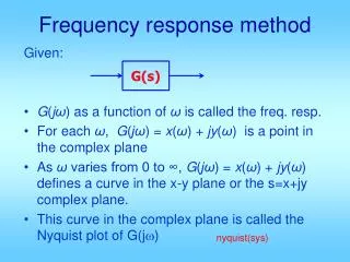
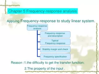
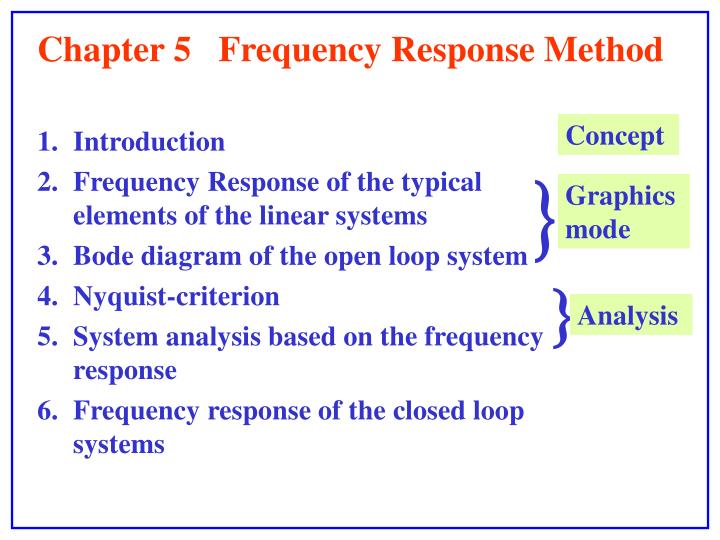
Concept . Graphics mode. Analysis . Chapter 5 Frequency Response Method. Introduction Frequency Response of the typical elements of the linear systems Bode diagram of the open loop system Nyquist-criterion System analysis based on the frequency response

E N D
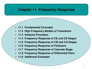
Concept Graphics mode Analysis Chapter 5 Frequency Response Method • Introduction • Frequency Response of the typical elements of the linear systems • Bode diagram of the open loop system • Nyquist-criterion • System analysis based on the frequency response • Frequency response of the closed loop systems
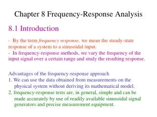
R We have the steady-state response: C uc ur 5.1 Introduction Three advantages: * Frequency response(mathematical modeling) can be obtained directly by experimental approaches. * easy to analyze the effects of the system with sinusoidal voices. * easy to analyze the stability of the systems with a delay element 5.1.1 frequency response For a RC circuit:
Make: then: We have: Here: We call: 5.1 Introduction Frequency Response(or frequency characteristic) of the electric circuit.
Definition:frequency response (or characteristic) —the ratio of the complex vector of the steady-state output versus sinusoid input for a linear system, that is: Here: (amplitude ratioof the steady-state output versus sinusoid input) 5.1 Introduction Generalize above discussion, we have: And we name: (phase differencebetween steady-state output and sinusoid input )
Input a sinusoid signal to the control system Measure the amplitude and phase of the steady-state output Change frequency Get the amplitude ratio of the output versus input Get the phase difference between the output and input N Are the measured data enough? y Data processing 5.1.2 approaches to get the frequency characteristics 1. Experimental discrimination
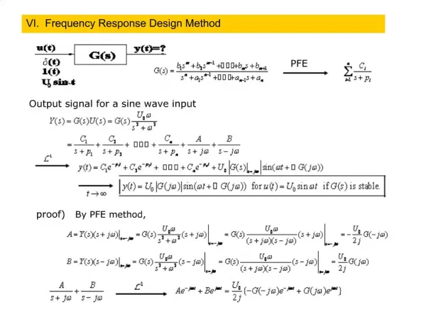
5.1.2 approaches to get the frequency characteristics 2. Deductive approach Theorem: If the transfer function is G(s), we have: Proof : Where — piis assumed to be distinct pole (i=1,2,3…n).
For the stable system all poles (-pi) have a negative real parts, we have the steady-state output signal: 5.1.2 approaches to get the frequency characteristics Taking the inverse Laplace transform:
Compare with the sinusoid input , we have: 5.1.2 approaches to get the frequency characteristics the steady-state output: Theamplitude ratio of the steady-state output cs(t) versus sinusoid input r(t): Thephase difference between the steady-state output and sinusoid input: Then we have :
a unity feedback control system, the open-loop transfer function: 1) Determine the steady-state response c(t) of the system. 2) Determine the steady-state error e(t) of the system. 5.1 Introduction Examples 5.1.1 Solution: 1) Determine the steady-state response c(t) of the system. The closed-loop transfer function is:
5.1 Introduction The frequency characteristic : The magnitude and phase response : The output response: So we have the steady-state response c(t) :
5.1 Introduction 2) Determine the steady-state error e(t) of the system. The error transfer function is : The error frequency response: The steady state error e(t) is:
5.1 Introduction Graphic expression —— for intuition 1. Rectangular coordinates plot 5.1.3 Graphic expressionof the frequency response Example 5.1.2
Calculate A(ω) and for different ω: Im Re -135o -117o 5.1.3 Graphic expression of the frequency response The polar plot is easily useful for investigating system stability. Example 5.1.3 2. Polar plot The magnitude and phase response:
Magnitude response — Y-coordinate in decibels: X-coordinate in logarithm of ω: logω Phase response — Y-coordinate in radian: X-coordinate in logarithm of ω: logω 5.1.3 Graphic expression of the frequency response Idea: How to enlarge the lower frequency band and shrink (shorten) the higher frequency band? The shortage of the polar plot and the rectangular coordinates plot: to synchronously investigate the cases of the lower and higher frequency band is difficult. 3. Bode diagram(logarithmic plots) Plot the frequency characteristic in a semilog coordinate: Firstwe discuss the Bode diagram in detail with the frequency response of the typical elements.
Im K Re 0dB, 0o 10 0.1 1 100 5.2 Frequency Response of The Typical Elements 1. Proportional element The typical elements of the linear control systems — refer to Chapter 2. Transfer function: Frequency response: Polar plot Bode diagram
Im Re 0dB, 0o 10 0.1 1 100 5.2 Frequency response of the typical elements Transfer function: Frequency response: 2. Integrating element Polar plot Bode diagram
Im 0dB, 0o 10 0.1 1 100 Re 1 5.2 Frequency response of the typical elements Transfer function: 3. Inertial element 1/T: break frequency Polar plot Bode diagram
maximum value of : 5.2 Frequency response of the typical elements Transfer function: 4. Oscillating element Make:
0dB, 0o 10 0.1 1 100 1 Im Re 5.2 Frequency response of the typical elements The polar plot and the Bode diagram: Polar plot Bode diagram
Im Im Im Re Re Re 5.2 Frequency response of the typical elements Transfer function: 5. Differentiating element 1 1 differential 1th-order differential 2th-order differential Polar plot
5.2 Frequency response of the typical elements Because of the transfer functions of the differentiating elements are the reciprocal of the transfer functions of Integrating element, Inertial element and Oscillating element respectively, that is: the Bode curves of the differentiating elements are symmetrical to the logω-axis with the Bode curves of the Integrating element, Inertial element and Oscillating element respectively. Then we have the Bode diagram of the differentiating elements:
0dB, 0o 10 0.1 1 100 0dB, 0o 10 0.1 1 100 0dB, 0o 10 0.1 1 100 5.2 Frequency response of the typical elements differential 2th-order differential 1th-order differential
Im 0dB, 0o Re 10 0.1 1 100 5.2 Frequency response of the typical elements Transfer function: 6. Delay element R=1 Polar plot Bode diagram
5.3 Bode diagram of the open loop systems 5.3.1 Plotting methods of the Bode diagram of the open loop systems Assume: We have: That is, Bode diagram of a open loop system is the superposition of the Bode diagrams of the typical elements. Example 5.3.1
① ② ③ ④ 0dB, 0o 10 0.1 1 100 ② 40dB, 90o ① 20dB, 45o ④ -20dB, -45o -40dB, -90o -60dB.-135o ③ -80dB,-180o 5.3 Bode diagram of the open loop systems G(s)H(s) could be regarded as: Then we have: 20dB/dec -40dB/dec -20dB/dec -20dB/dec -40dB/dec -40dB/dec
5.3.2 Facility method to plot the magnitude response of the Bode diagram Summarizing example 5.3.1, we have the facility method to plot the magnitude response of the Bode diagram: 1) Mark all break frequencies in theω-axis of the Bode diagram. 2) Determine the slope of the L(ω) of the lowest frequency band (before the first break frequency) according to the number of the integrating elements: -20dB/dec for 1 integrating element -40dB/dec for 2 integrating elements … 3) Continue the L(ω) of the lowest frequency band until to the first break frequency, afterwards change the the slope of the L(ω) which should be increased 20dB/dec for the break frequency of the 1th-order differentiating element . The slope of the L(ω) should be decreased 20dB/dec for the break frequency of the Inertial element …
5.3.2 Facility method to plot the magnitude response of the Bode diagram Plot the L(ω) of the rest break frequencies by analogy . Example 5.3.2 The Bode diagram is shown in following figure:
-20dB/dec 1.25dB 0dB, 0o 10 0.1 1 100 40dB, 90o 20dB, 45o -20dB, -45o -40dB, -90o -60dB.-135o -100dB,-225o -80dB,-180o -120dB,-270o 5.3.2 Facility method to plot the magnitude response of the Bode diagram -20dB/dec -60dB/dec There is a resonant peak Mr at:
We have: 5.3.3 Determine the transfer function in terms of the Bode diagram Compare following transfer functions: • The minimum phase system(or transfer function) The magnitude responses are the same. But the net phase shifts are different when ω vary from zero to infinite. It can be illustrated as following: Sketch the polar plot:
Im Re It is obvious: the net phase shifts of the Im G1(jω) is the minimum when ω vary from zero to infinite. Im Re Re G1(s) is named: the minimum phase transfer function . 5.3.3 Determine the transfer function in terms of the Bode diagram Im The polar plot: Re phase shift -π phase shift 00 phase shift -π phase shift π
5.3.3 Determine the transfer function of the minimum phase systemsin terms of the magnitude response A transfer function is called a minimum phase transfer func- tion if its zeros and poles all lie in the left-hand s-plane. A transfer function is called a non-minimum phase transfer function if it has any zero or pole lie in the right-hand s-plane. Only for the minimum phase systems we can affirmatively deter- mine the relevant transfer function from the magnitude response of the Bode diagram . Definition: 2. Determine the transfer function from the magnitude response of the Bode diagram . Example 5.3.3
20dB 20dB/dec -20dB/dec 0.5 200 0dB 0dB, 0o 10 10 0.1 0.1 1 1 100 100 -40dB/dec -20dB/dec -40dB/dec 5.3.3 Determine the transfer function in terms of the Bode diagram 2 20 200 Example 5.3.4
20dB 20dB/dec -20dB/dec 0.5 200 0dB 0dB 10 0.1 0.1 1 1 100 10 100 -20dB/dec 8.136 dB 20 dB -60dB/dec -20dB/dec 5.3.3 Determine the transfer function in terms of the Bode diagram Example 5.3.5
0dB 0.1 1 10 100 -20dB/dec 8.136 dB 20 dB -60dB/dec -20dB/dec 5.3.3 Determine the transfer function in terms of the Bode diagram For the non-minimum phase system we must combine the magnitude response and phase response together to determine the transfer function.
-20dB/dec -90o -180o 0dB, 0o 100 0.1 10 1 5.3.3 Determine the transfer function in terms of the Bode diagram Example 5.3.6 All satisfy the magnitude response But
5.4 The Nyquist-criterion 5.4.1 The argument principle(Cauchy’s theorem) A method to investigate the stability of a system in terms of the open-loop frequency response. Assume: Make : Note: si→the zeros of the F(s), also the roots of the 1+G(s)H(s)=0
Now we consider the net phase shift if s travels 360o along a closed path Γ of the s-plane in the clockwise direction shown in Fig.5.4.1 . Im Re 5.4.1 The argument principle S-plane Similarly we have: Fig. 5.4.1
If a closed path Γ in the s-plane encircles Z zeros and P poles of F(s) and does not pass through any poles or zeros of F(s) , when s travels along the contour Γ in the clockwise direction, the corres- ponding F(s) locus mapped in the F(s)-plane will encircle the origin of the F(s) plane N = P-Z times in the counterclockwise direction, that is: 5.4.1 The argument principle If Z zeros and P poles are enclosed by Γ , then: It is obvious that path Γ can not pass through any zeros sior poles pj . Then we have the argument principle: N = P - Z
Im Re S-plane Fig. 5.4.2 5.4.1 The argument principle P —— number of the zeros of the F(s) encircled by the path Γ in the s-plane. Z —— number of the poles of the F(s) encircled by the path Γ in the s-plane. here: N —— number of the F(s) locus encircling the origin of the F(s)-plane in the counterclockwise direction. 5.4.2 Nyquist criterion If we choose the closed path Γ so thatthe Γ encircles the entire right hand of the s-plane but not pass through any zeros or poles of F(s) shown in Fig.5.4.2 . The path Γ is called the Nyquist-path.
Im Re S-plane 5.4.2 Nyquist criterion When s travels along the the Nyquist-path: Because the origin of the F(s)-plane is Fig. 5.4.2 equivalent to the point (-1, j0) of the G(jω)H(jω)-plane, we have another statement of the argument principle: When ω vary from - (or 0) →+ , G(jω)H(jω) Locus mapped in the G(jω)H(jω)-plane will encircle the point (-1, j0) in the counterclockwise direction: here: P — the number of the poles of G(s)H(s) in the right hand of the s-plane. Z — the number of the zeros of F(s) in the right hand of the s-plane.
5.4.2 Nyquist-criterion If the systems are stable, should be Z = 0, then we have: The sufficient and necessary condition of the stability of the linear systems is :When ω vary from - (or 0) →+ , the G(jω)H(jω)Locus mapped in theG(jω)H(jω)-plane will encircle the point (-1, j0) as P (or P/2) times in the counterclockwise direction. ——Nyquist criterion Here: P — the number of the poles of G(s)H(s) in the right hand of the s-plane. Discussion : i) If the open loop systems are stable, that is P = 0, then: for the stable open-loop systems, The sufficient and necessary condition of the stability of the closed-loop systems is : When ω vary from - (or 0) →+ , the G(jω)H(jω) locus mapped in the G(jω)H(jω)-plane will not encircle the point (-1, j0).
5.4.2 Nyquist-criterion G(jω)H(jω) Locus traverses the left real axis of the point (-1, j0) in the counterclockwise direction —“positive traversing”. ii) Because that the G(jω)H(jω) locus encircles the point (-1, j0) means that the G(jω)H(jω) locus traverse the left real axis of the point (-1, j0) , we make: G(jω)H(jω) Locus traverses the left real axis of the point (-1, j0) in the clockwise direction —“negative traversing”. Then we have another statement of the Nyquist criterion: The sufficient and necessary condition of the stability of the linear systems is :When ω vary from - (or 0) →+ , the number of the net “positive traversing” is P (orP/2). Here: the net “positive traversing” —— the difference between the number of the “positive traversing” and the number of the “negative traversing” .
(-1, j0) (-1, j0) Im Im Im Im (1) P=2 Re Re Re Re (2) P=0 (-1, j0) (-1, j0) (3) P=2 (4) P=0 5.4.2 Nyquist-criterion The polar plots of the open loop systems are shown in Fig.5.4.3, determine whether the systems are stable. Example 5.4.1 stable stable unstable unstable Fig.5.4.3
We consider a semicircular detour around the pole (s = 0) repre-sented by setting -2 -1 5.4.2 Nyquist-criterion the system with the poles (or zeros) at the imaginary axis Example 5.4.2 There is a pole s = 0 at the origin in this system, but the Nyquist path can not pass through any poles of G(s)H(s). Note: Idea: Im at the s = 0 point we have: Re Fig. 5.4.4
Im Re Im Re (-1, j0) Fig. 5.4.4 5.4.2 Nyquist-criterion It is obvious that there is a phase saltation of the G(jω)H(jω) at ω=0, and the magnitude of the G(jω)H(jω) is infinite at ω=0. Fig.5.4.5 In terms of above discussion , we can plot the system’s polar plot shown as Fig.5.4.5. The closed loop system is unstable.
Im Re (-1, j0) Fig.5.4.6 Example 5.4.3 Determine the stability of the system applying Nyquist criterion. Solution Similar to theExample 5.4.2, the system’s polar plot is shown as Fig.5.4.6 . The closed loop system is unstable. 5.4.3 Application of the Nyquist criterion in the Bode diagram
5.4.3 Application of the Nyquist criterion in the Bode diagram G(jω)H(jω)locus traverses the left real axis of the point (-1, j0) in G(jω)H(jω)-plane→L(ω)≥0dB and φ(ω) =-180o in Bode diagram (as that mentioned in 5.4.2). We havethe Nyquist criterion in the Bode diagram: The sufficient and necessary condition of the stability of the linear closed loop systems is :When ω vary from 0→+ , the number of the net “positive traversing” is P/2. Here:the net “positive traversing” —the difference between the number of the “positive traversing” and the number of the “negative traversing” in all L(ω)≥0dB ranges of the open-loop system’s Bode diagram. “positive traversing”— φ(ω) traverses the “-180o line” from below to above in the open-loop system’s Bode diagram; “negative traversing”— φ(ω) traversesthe “-180o line” from above to below.
-20 -40 -90o -60 φ(ω) -40 -20 0dB, -180o -40 -60 -270o L(ω) Fig.5.4.7 5.4.3 Application of the Nyquist criterion in the Bode diagram The Bode diagram of a open-loop stable system is shown in Fig.5.4.7, determine whether the closed loop system is stable. Solution Example 5.4.4 Because the open-loop system is stable, P = 0 . In terms of the Nyquist criterion in the Bode diagram: The number of the net “positive traversing” is 0 ( = P/2 = 0 ). The closed loop system is stable .
5.4.4 Nyquist criterion and the relative stability (Relative stability of the control systems) In frequency domain, the relative stability could be described by the “gain margin” and the “phase margin”. 1. Gain margin Kg 2. Phase margin γc 3. Geometrical and physical meanings of the Kg and γc