Download
1 / 20
230 likes | 558 Views
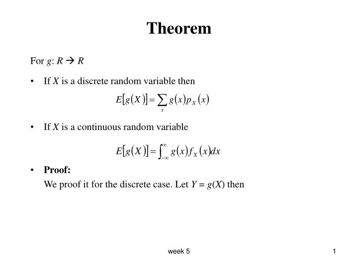
Theorem. For g : R R If X is a discrete random variable then If X is a continuous random variable Proof: We proof it for the discrete case. Let Y = g ( X ) then. Example to illustrate steps in proof. Suppose i.e. and the possible values of X are

E N D
Theorem For g: RR • If X is a discrete random variable then • If X is a continuous random variable • Proof: We proof it for the discrete case. Let Y = g(X) then week 5
Example to illustrate steps in proof • Suppose i.e. and the possible values of X are so the possible values of Y are then, week 5
Examples 1. Suppose X ~ Uniform(0, 1). Let then, 2. Suppose X ~ Poisson(λ). Let , then week 5
Properties of Expectation For X, Y random variables and constants, • E(aX + b) = aE(X) + b Proof: Continuous case • E(aX + bY) = aE(X) + bE(Y) Proof to come… • If X is a non-negative random variable, then E(X) = 0 if and only if X = 0 with probability 1. • If X is a non-negative random variable, then E(X) ≥ 0 • E(a) = a week 5
Moments • The kth moment of a distribution is E(Xk). We are usually interested in 1st and 2nd moments (sometimes in 3rd and 4th) • Some second moments: 1. Suppose X ~ Uniform(0, 1), then 2. Suppose X ~ Geometric(p), then week 5
Variance • The expected value of a random variable E(X) is a measure of the “center” of a distribution. • The variance is a measure of how closely concentrated to center (µ) the probability is. It is also called 2nd central moment. • Definition The variance of a random variable X is • Claim: Proof: • We can use the above formula for convenience of calculation. • The standard deviation of a random variable X is denoted by σX ; it is the square root of the variance i.e. . week 5
Properties of Variance For X, Y random variables and are constants, then • Var(aX + b) = a2Var(X) Proof: • Var(aX + bY) = a2Var(X) + b2Var(Y) + 2abE[(X – E(X ))(Y – E(Y ))] Proof: • Var(X) ≥ 0 • Var(X) = 0 if and only if X = E(X) with probability 1 • Var(a) = 0 week 5
Examples 1. Suppose X ~ Uniform(0, 1), then and therefore 2. Suppose X ~ Geometric(p), then and therefore 3. Suppose X ~ Bernoulli(p), then and therefore, week 5
Example • Suppose X ~ Uniform(2, 4). Let . Find . • What if X ~ Uniform(-4, 4)? week 5
Functions of Random variables • In some case we would like to find the distribution of Y = h(X) when the distribution of X is known. • Discrete case • Examples 1. Let Y = aX + b , a≠ 0 2. Let week 5
Continuous case – Examples 1. Suppose X ~ Uniform(0, 1). Let , then the cdf of Y can be found as follows The density of Y is then given by 2. Let X have the exponential distribution with parameter λ. Find the density for 3. Suppose X is a random variable with density Check if this is a valid density and find the density of . week 5
Question • Can we formulate a general rule for densities so that we don’t have to look at cdf? • Answer: sometimes … Suppose Y = h(X) then and but need h to be monotone on region where density for X is non-zero. week 5
Check with previous examples: 1. X ~ Uniform(0, 1) and 2. X ~ Exponential(λ). Let 3. X is a random variable with density and week 5
Theorem • If X is a continuous random variable with density fX(x) and h is strictly increasing and differentiable function form RR then Y = h(X) has density for . • Proof: week 5
Theorem • If X is a continuous random variable with density fX(x) and h is strictly decreasing and differentiable function form RR then Y = h(X) has density for . • Proof: week 5
Summary • If Y = h(X) and h is monotone then • Example X has a density Let . Compute the density of Y. week 5
Indicator Functions and Random Variables • Indicator function – definition Let A be a set of real numbers. The indicator function for A is defined by • Some properties of indicator functions: • The support of a discrete random variable X is the set of values of x for which P(X = x) > 0. • The support of a continuous random variable X with density fX(x) is the set of values of x for which fX(x) > 0. week 5
Examples • A discrete random variable with pmf can be written as • A continuous random variable with density function can be written as week 5
Important Indicator random variable • If A is an event then IA is a random variable which is 0 if A does not occur and 1 if it does. IA is an indicator random variable. IA is also called a Bernoulli random variable. • If we perform a random experiment repeatedly and each time measure the random variable IA, we could get 1, 1, 0, 0, 0, 0, 1, 0, …The average of this list in the long run is E(IA); it gives the proportion with which A occurs. In the long run it is P(A), i.e. P(A) = E(IA) • Example: for a Bernoulli random variable X we have week 5
Use of Indicator random variable • Suppose X ~ Binomial(n, p). Let Y1,…, Yn be Bernoulli random variables with probability of success p. Then X can be thought of as , then • Similar trick for Negative Binomial: Suppose X ~ Negative Binomial(r, p). Let X1 be the number of trials until the 1st success X2 be the number of trails between 1st and 2nd success . : Xr be the number of trails between (r - 1)th and rth success Then and we have week 5