Viola-Jones Face Detection Algorithm

1. Learning to Detect FacesA Large-Scale Application of Machine Learning(This material is not in the text: for further information see the paper by P. Viola and M. Jones, International Journal of Computer Vision, 2004

2. Viola-Jones Face Detection Algorithm • Overview : • Viola Jones technique overview • Features • Integral Images • Feature Extraction • Weak Classifiers • Boosting and classifier evaluation • Cascade of boosted classifiers • Example Results

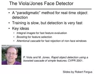
3. Viola Jones Technique Overview • Three major contributions/phases of the algorithm : • Feature extraction • Learning using boosting and decision stumps • Multi-scale detection algorithm • Feature extraction and feature evaluation. • Rectangular features are used, with a new image representation their calculation is very fast. • Classifier learning using a method called boosting • A combination of simple classifiers is very effective

4. Features • Four basic types. • They are easy to calculate. • The white areas are subtracted from the black ones. • A special representation of the sample called the integral image makes feature extraction faster.

5. Integral images • Summed area tables • A representation that means any rectangle’s values can be calculated in four accesses of the integral image.

6. Fast Computation of Pixel Sums

7. Feature Extraction • Features are extracted from sub windows of a sample image. • The base size for a sub window is 24 by 24 pixels. • Each of the four feature types are scaled and shifted across all possible combinations • In a 24 pixel by 24 pixel sub window there are ~160,000 possible features to be calculated.

8. Learning with many features • We have 160,000 features – how can we learn a classifier with only a few hundred training examples without overfitting? • Idea: • Learn a single very simple classifier (a “weak classifier”) • Classify the data • Look at where it makes errors • Reweight the data so that the inputs where we made errors get higher weight in the learning process • Now learn a 2nd simple classifier on the weighted data • Combine the 1st and 2nd classifier and weight the data according to where they make errors • Learn a 3rd classifier on the weighted data • … and so on until we learn T simple classifiers • Final classifier is the combination of all T classifiers • This procedure is called “Boosting” – works very well in practice.

9. “Decision Stumps” • Decision stumps = decision tree with only a single root node • Certainly a very weak learner! • Say the attributes are real-valued • Decision stump algorithm looks at all possible thresholds for each attribute • Selects the one with the max information gain • Resulting classifier is a simple threshold on a single feature • Outputs a +1 if the attribute is above a certain threshold • Outputs a -1 if the attribute is below the threshold • Note: can restrict the search for to the n-1 “midpoint” locations between a sorted list of attribute values for each feature. So complexity is n log n per attribute. • Note this is exactly equivalent to learning a perceptron with a single intercept term (so we could also learn these stumps via gradient descent and mean squared error)

10. Boosting Example

11. First classifier

12. First 2 classifiers

13. First 3 classifiers

14. Final Classifier learned by Boosting

15. Final Classifier learned by Boosting

16. Boosting with Decision Stumps • Viola-Jones algorithm • With K attributes (e.g., K = 160,000) we have 160,000 different decision stumps to choose from • At each stage of boosting • given reweighted data from previous stage • Train all K (160,000) single-feature perceptrons • Select the single best classifier at this stage • Combine it with the other previously selected classifiers • Reweight the data • Learn all K classifiers again, select the best, combine, reweight • Repeat until you have T classifiers selected • Very computationally intensive • Learning K decision stumps T times • E.g., K = 160,000 and T = 1000

17. How is classifier combining done? • At each stage we select the best classifier on the current iteration and combine it with the set of classifiers learned so far • How are the classifiers combined? • Take the weight*feature for each classifier, sum these up, and compare to a threshold (very simple) • Boosting algorithm automatically provides the appropriate weight for each classifier and the threshold • This version of boosting is known as the AdaBoost algorithm • Some nice mathematical theory shows that it is in fact a very powerful machine learning technique

18. Reduction in Error as Boosting adds Classifiers

19. Useful Features Learned by Boosting

20. A Cascade of Classifiers

21. Detection in Real Images • Basic classifier operates on 24 x 24 subwindows • Scaling: • Scale the detector (rather than the images) • Features can easily be evaluated at any scale • Scale by factors of 1.25 • Location: • Move detector around the image (e.g., 1 pixel increments) • Final Detections • A real face may result in multiple nearby detections • Postprocess detected subwindows to combine overlapping detections into a single detection

22. Training • Examples of 24x24 images with faces

23. Small set of 111 Training Images

24. Sample results using the Viola-Jones Detector • Notice detection at multiple scales

25. More Detection Examples

26. Practical implementation • Details discussed in Viola-Jones paper • Training time = weeks (with 5k faces and 9.5k non-faces) • Final detector has 38 layers in the cascade, 6060 features • 700 Mhz processor: • Can process a 384 x 288 image in 0.067 seconds (in 2003 when paper was written)