Download
1 / 32
320 likes | 406 Views
3-D Reconstruction of the Inner Heliosphere from Remote-Sensing Data: A Global Solar Wind Boundary that Includes CME Transient Effects. B.V. Jackson , H-S Yu, P.P. Hick, A. Buffington Center for Astrophysics and Space Sciences, University of California at San Diego, LaJolla, CA, USA.

E N D
3-D Reconstruction of the Inner Heliosphere from Remote-Sensing Data: A Global Solar Wind Boundary that Includes CME Transient Effects B.V. Jackson, H-S Yu, P.P. Hick, A. Buffington Center for Astrophysics and Space Sciences, University of California at San Diego, LaJolla, CA, USA Masayoshi http://smei.ucsd.edu/ http://ips.ucsd.edu/
Introduction: The Motive: To Provide a Boundary for MHD and Kinematic Solar Wind Models. The Analysis: 3-D Heliospheric Tomography – (a fit to data) (Time-dependent view from a single observer location) The Current Data Sets: IPS (STELab, Ooty, MEXART?), SMEI This Project: An analysis that includes in-situ data and a magnetic field potential field extrapolation from the solar surface.
DATA STELab IPS Heliospheric Analyses IPS line-of-sight response STELab IPS array near Mt. Fuji STELab IPS array systems
Current STELab IPS Heliospheric Analyses New STELab IPS array in Toyokawa (3,432 m2 array now operates well – year-round operation began in 2011)
Other Current IPS Radio Systems The Ootacamund (Ooty), India off-axis parabolic cylinder 530 m long and 30 m wide (15,900 m2) operating at a nominal frequency of 326.5 MHz. MEXART IPS 9,600 m2 140 MHz IPS radio array near Michoacan, Mexico
The Solar Mass Ejection Imager (SMEI) Jackson, B.V., et al., 2004, Solar Phys., 225, 177 Launch 6 January 2003 Closure 28 Sept 2011 Sun C1 C2 C3 Sun 1 gigabyte/day; total ~4 terabytes Simultaneous images from the three SMEI cameras.
Frame Composite for Aitoff Map Blue = Cam3; Green= Cam2; Red = Cam1 D290; 17 October 2003
SMEI first light composite image Composite all-sky map 2 Feb 2003 from the three SMEI cameras.
Heliospheric 3-D Reconstruction Jackson, B.V., et al., 2008, Adv. in Geosciences, 21, 339 The outward-flowing solar wind structure follows very specific physics as it moves outward from the Sun LOS Weighting
Jackson, B.V., et al., 2008, Adv. in Geosciences, 21, 339 Relative Weighting Outward Radial Motion
Jackson, B.V., et al., 2008, Adv. in Geosciences, 21, 339. The UCSD 3D-reconstruction program The “traceback matrix”(any solar wind model works)In the traceback matrix the location of the upper level data point (starred) is an interpolation in x of Δx2 and the unit x distance – Δx3 distance or (1 – Δx3). Similarly, the value of Δt at the starred point is interpolated by the same spatial distance. Each 3D traceback matrix contains a regular grid of values ΣΔx, ΣΔy, ΣΔt, ΣΔv, and ΣΔm that locates the origin of each point in the grid at each time and its change in velocity and density from the heliospheric model.
Heliospheric 3-D Reconstruction Jackson, B.V., et al., 2008, Adv. in Geosciences, 21, 339. Line of sight “crossed” components on a reference surface. Projections on the reference surface are shown. These weighted components are inverted to provide the time-dependent tomographic reconstruction. 13 July 2000 14 July 2000
Jackson, B.V., et al., 2010,Solar Phys., 265, 245-256. IPS line-of-sight response Jackson, B.V., et al., 2008, Adv. in Geosciences, 21, 339. The inclusion of in-situ data provides a more stable 3D reconstruction solution globally, and allows a better interpolation across time intervals without much remote-sensing data. Innovation STELab IPS * 13 July 2000 Inclusion of in-situ measurements into the 3D-reconstructions
2011/11/09 CME LASCO C2 COR2 B
2011/11/09 CME (Forecast) LASCO C2 IPS Image of Event
2011/11/09 CME (Forecast) LASCO C2 IPS Remote-Observer View
Jackson, B.V., et al., 2008, Adv. in Geosciences, 21, 339. Jackson, B.V., et al., 2012, Solar Phys., published on-line. IPS C.A.T. Analysis (Forecast) 2011/11/09 CME Density Ecliptic Cut Density Meridional Cut
IPS C.A.T. Analysis Jackson, B.V., et al., 2008, Adv. in Geosciences, 21, 339. Jackson, B.V., et al., 2012, Solar Phys., published on-line. IPS C.A.T. Analysis (Forecast) (Forecast) 2011/11/09 CME Forecast Density Ecliptic Cut Density Forecast at 1AU
IPS C.A.T. Analysis Jackson, B.V., et al., 2008, Adv. in Geosciences, 21, 339. Jackson, B.V., et al., 2012, Solar Phys., published on-line. IPS C.A.T. Analysis (Forecast) (Forecast) 2011/11/09 CME Boundary Forecast Velocity Ecliptic Cut Velocity Forecast at 1AU
Zhao, X. P. and Hoeksema, J. T., 1995, J. Geophys. Res., 100 (A1), 19. http://ips.ucsd.edu/ Magnetic Field Extrapolation Dunn et al., 2005, Solar Physics 227: 339–353. • Inner region: the CSSS model calculates the magnetic field usingphotospheric measurements and a horizontal current model. 2. Middle region: the CSSS model opens the field lines. In the outer region. 3. Outer region: the UCSD tomography convects the magnetic field along velocity flow lines. Jackson, B.V., et al., 2012, Adv. in Geosciences, 30, 93-115.
How to Extrapolate Across Data Outages Type of Outage (hierarchy) Too Few Lines of Sight on Any Given Day Interpolate using a spatial & temporal co-rotation “fill in” Few Days Interpolate using a spatial & temporal co-rotation “fill in” Weeks Interpolate using a temporalco-rotation “fill in” Months (IPS 3-site data not obtained in winter) Interpolate V using in-situ ecliptic measurements
To Make a 3D-MHD Boundary Time-Dependent Velocity at 0.25 AU, IHG Coordinates ACE in-situ Measurement Inclusion
To Make a 3D-MHD Boundary Time-Dependent Density at 0.25 AU, IHG Coordinates ACE in-situ Measurement Inclusion
To Make a 3D-MHD Boundary Time-Dependent Radial Field at 0.25 AU, IHG Coordinates ACE in-situ Measurement Inclusion
Heliospheric 3D-reconstructions Lan Jian CCMC Study CR 2056-2063 In-SituTomographic analysis
Heliospheric 3D-reconstructions Lan Jian CCMC Study CR 2056-2063 In-SituTomographic analysis
Heliospheric 3D-reconstructions Lan Jian CCMC Study CR 2056-2063 In-SituTomographic analysis
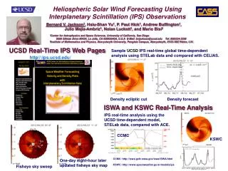
Jackson, B.V., et al., 2012, Adv. in Geosciences, 30, 93-115. http://ips.ucsd.edu/ UCSD Web pages UCSD IPS analysis Web Analysis Runs Automatically Using Linux on a P.C.
Summary: The analysis of IPS data provides low-resolution global measurements of density and velocityinter-mediate between Sun and Earth with a time cadence of one day for both density and velocity, and slightly longer cadences for some magnetic field components. There are several near real time and archival data sources (IPS, SMEI), but the most long-term and substantiated data source (that also measures velocity globally) is IPS data from the STELab arrays in Japan. Accurate observations of inner heliosphere parameters coupled withthe best physicscan extrapolate these outward to Earth or the interstellar boundary.
Density Turbulence • Scintillation index, m, is a measure of level of turbulence • Normalized Scintillation index, g = m(R) / <m(R)> • g > 1 enhancement in Ne • g 1 ambient level of Ne • g < 1 rarefaction in Ne (CourtesyofP.K.Manoharan) A scintillation enhancement with respect to the ambient wind identifies the presence of a region of increased turbulence/density and a possible CME along the line-of-sight to the radio source.
Jackson, B.V., et al., 2012, Solar Phys., (under review). Density analysis for all of CR 2114 IPS time series – time of tomographic run compared to ACE one day in advance Correlation
Jackson, B.V., et al., 2012, Solar Phys., (under review). Analysis CR 2110 – CR 2116 (spring – winter 2011) IPS time series compared to ACE