Download
1 / 51
520 likes | 542 Views
Formal Models of Computation. Turing Machines. Turing Machines. Abstract but accurate model of computers Proposed by Alan Turing in 1936 There weren ’ t computers back then!

E N D
Formal Models of Computation Turing Machines
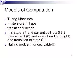
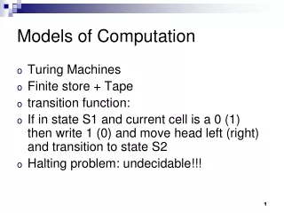
Turing Machines • Abstract but accurate model of computers • Proposed by Alan Turing in 1936 • There weren’t computers back then! • Turing’s motivation: find out whether there exist mathematical problems that cannot be solved algorithmically. (This is Hilbert’s “Entscheidungsproblem”, i.e., decision problem) • Similar to a FSA but with an • Unlimited and unrestricted memory • Able to do everything a real computer can do • However: • There are problems even a Turing Machine (TM) can’t solve! • Such problems are beyond the theoretical limits of computation formal models of computation
Turing Machines: Features Control Head . . . Tape a b a a □ □ □ • A tape is a countably infinite list of cells • A tape head can • read and write symbols from/onto a cell on the tape • move forward and backward on the tape • Schematically: formal models of computation
Turing Machines: Features (Cont’d) • Initially the tape • Contains only the input string • Is blank everywhere else • If the TM needs to store information • It can write it onto the tape • To read the info it has written • TM can move the head back over it • TMs have the following behaviours: • They “compute” then stop in a “reject” state • They “compute” then stop in an “accept” state • They loop forever • Compare FSAs: These have no “reject” states, and no looping forever. (Why not?) formal models of computation
Turing Machines vs. Finite Automata • TMs can both write on the tape and read from it • FSAs can only read (or only write if they are generators) • The read/write head can move to the left and right • FSAs cannot “go back” on the input • The tape is infinite • In FSAs the input and output is always finite • The accept/reject states take immediate effect • There is no need to “consume” all the input • TMs come in different flavours.There differences are unimportant. formal models of computation
Turing Machine: an informal Example • TM M1 to test if an input (on the tape) belongs to B = {w#w | w {0,1}* } M1 checks if the contents of the tape consists of two identical strings of 0’s & 1’s separated by “#” • M1 accepts inputs 0110#0110, 000#000, 010101010#010101010 • M1 rejects inputs 1111#0000, 000#0000, 0001#1000 • M1 should work for any size of input (general) • There are infinitely many, so we cannot use “cases” • How would you program this? • All you have is a tape, and a head to read/write it formal models of computation
Turing Machine: an Example (Cont’d) • Strategy for M1: • “Zig-zag” to corresponding places at both sides of “#” and check if they match • Mark (cross off) those places you have checked • If it crosses off all symbols, then everything matches and M1 goes into an accept state • If it discovers a mismatch then it enters a reject state formal models of computation
Turing Machine: an Example (Cont’d) • M1 = “On input string S • Scan the input to be sure it contains a single # symbol; if not, reject. • Zig-zag across the tape to corresponding positions on either side of # to check if they contain the same symbol. • If they do not match, reject. • Cross off symbols as they are checked to keep track of things. • When all symbols to the left of # have been crossed off, check for any remaining symbols to the right of #. • If any symbols remain, reject; otherwise accept.” formal models of computation
Turing Machine: an Example (Cont’d) x x x x 0 x x 1 x x 1 x 1 1 1 1 1 x 1 1 1 0 0 x 0 0 0 0 0 0 0 x 0 0 0 0 x 0 0 0 0 0 # # # # # # # x 0 x 0 x x x 1 x x 1 1 1 1 1 1 1 1 x 1 1 x 0 0 0 0 0 0 0 0 x 0 0 0 0 0 x 0 0 0 0 0 . . . . . . . . . . . . . . . . . . . . . □ □ □ □ □ □ □ • Snapshots of M1’s tape during stages 2 and 3: . . . Accept!! formal models of computation
Formal Definition of Turing Machines • Previous slides give a flavour of TMs, but not their details. • We can describe TMs formally, similarly to what you did for FAs • We shall not always use formal descriptions for TMs because these would tend to be quite long • but ultimately, our informal descriptions should be “translatable” into formal ones • so it is crucial to understand these formal descriptions formal models of computation
Formal definition of Turing Machines • The imperative model of “algorithmhood” is formulated in terms of actions: • A TM is always in one of a specified number of states (these include the accept and reject states) • The action of the TM, at a given moment, depends on its state and on what the TM is reading at that moment • Always perform three types of actions: (1) replace the symbol that it reads by another (or the same) symbol, (2) move the head Left or Right, and (3) enter a new state (or the same state again). formal models of computation
Formal Definition of TMs (Cont’d) • The heart of a TM is a function mapping • A state s of the machine • The symbol a on the tape where the head is onto • A new state t of the machine • A symbol b to be written on the tape (over a) • A movement L (left) or R (right) of the head That is, (s,a) = (t,b,L) “When the machine is in state s and the head is over a cell containing a symbol a, then the machine writes the symbol b (replacing a), goes to state t and moves the head to the Left.” formal models of computation
Formal Definition of TMs (Cont’d) A Turing Machine is a 7-tuple (Q, , , , q0, qacc, qrej ) where Q, , are all finite sets and • Q is the set of states • is the input alphabetnot containing the special blank symbol “□” • is the tape alphabet, where {□} • :QQ{L,R} is the transition function • q0Q is the start state • qaccQ is the accept state • qrej Q is the reject state, where qrej qacc formal models of computation
How Turing Machines “Compute” M = (Q, , , , q0, qacc, qrej ) • M receives its input w=w1w2…wn * • w is on the leftmostn cells of the tape. • The rest of the tape is blank (infinite list of “□”) • The head starts on the leftmost cell of the tape • does not contain “□”, so the first blank on the tape marks the end of the input • M follows the “moves” encoded in • If M tries to move its head to the left of the left-hand end of the tape, the head stays in the same place • The computation continues until it enters the accept or reject state, at which point Mhalts • If neither occurs, M goes on forever… formal models of computation
Formalisation of TMs • Formalisation is needed to say precisely how TMs behave. For instance, • TMs use “sudden death” (and “sudden life”) • FSA accepts a string iff the (complete!) string is the label of a successful path. • TM accepts a string if, while processing it, an accept state is reached; TM rejects a string if, while processing it, a reject state is reached • What exactly does it mean to “move to the right”? • What if the head is already at the rightmost edge? formal models of computation
Configurations of TMs These three items are a configuration of the TM q7 . . . 1 0 1 1 0 1 1 1 1 1 □ □ □ • As a TM computes, changes occur in its: • State • Tape contents • Head location • Configurations are represented in a special way: • When the TM is in state q, and • The contents of the tape is two strings uv, and • The head is on the leftmost position of string v • Then we represent this configuration as “uqv” • Example: 1011q7011111 formal models of computation
Formalising TMs Computations qi qj a v a v . . . . . . u b u c □ □ Assume • a, b, c in (3 characters from the tape) • u and v in * (2 strings from the tape) • states qi and qj We can now say that (for all u and v) uaqibvyieldsuqjacv if (qi,b) = (qj,c,L) Graphically: formal models of computation
Formalising TMs Computations (Cont’d) qj a v u c qi a v . . . . . . u b □ □ A similar definition for rightward moves uaqibvyieldsuacqjv if (qi,b) = (qj,c,R) Graphically: formal models of computation
Formalising TMs Computations (Cont’d) qi qi qj qj v v v v b b c c . . . . . . . . . . . . □ □ □ □ • Special cases when head at beginning of tape • For the left-hand end, moving left: qibvyieldsqjcv if (qi,b) = (qj,c,L) • We prevent the head from “falling off” the left-hand end of the tape: • For the left-hand end, moving right: qibvyieldscqjv if (qi,b) = (qj,c,R) formal models of computation
Formalising TMs Computations (Cont’d) • For the right-hand “end” (not really the end…) • infinite sequence of blanks follows the part of the tape represented in the configuration • We thus handle the case above as any other rightward move formal models of computation
Formalising TMs Computations (Cont’d) • The start configuration of M on input w is q0w • M in start state q0 with head at leftmost position of tape • An accepting configuration has state qacc • A rejecting configuration has state qrej • Rejecting and accepting configurations are haltingconfigurations • They do not yield further configurations • No matter what else is in the configuration! • Note: is a function, and there is only one start state, so the TM (as defined here) is deterministic formal models of computation
Formalising TMs Computations (Cont’d) • A TM Maccepts input w if there is a sequence of configurations C1,C2,…,Ck where 1. C1 is the start configuration of M on input w 2. Each Ci yields Ci +1, and 3. Ck is an accepting configuration Analogous to FSAs, • the set of strings that M accepts is the language of M, denoted L(M) • we also say that a TM “accepts” or “recognizes” a language. formal models of computation
Sample Turing Machine (Cont’d) q1 q3 q2 q4 0 □,R 0 R Some shorthands to simplify notation: “when in state q1 with the head reading 0, it goes to state q2, writes □ and moves the head to the right” “machine moves its head to the right when reading 0 in the state q3, but nothing is written onto the tape” Transitions from accept/reject states can be omitted (because of sudden death). (q1,0) = (q2,□,R) (q3,0) = (q4,0,R) formal models of computation
First TM example • Given: w is a bitstring • Construct TM that recognises L={w: w contains at least one 0} formal models of computation
A very simple TM (diagram and formal) • Given: w is a bitstring • Construct TM that recognises L={w: w contains at least one 0} 0 R q0 Acc 1R □R Rej formal models of computation
First TM example (diagram and formal) • Given: w is a bitstring • Construct TM that recognises L={w: w contains at least one 0} 0 R q0 Acc 1R □R Rej Using formal notation: d(q0,1)=(q0,1,R). d(q0,0)=(Acc,0,R). d(q0,□)=(Rej, □,R) formal models of computation
Observe .. • The “transition function” in this graph is not a total function. However, • The missing arrows (from the Acc and Rej states) can easily be added • How you do this does not affect the language recognised by the TM formal models of computation
Second TM example • How would you modify the previous TM to recognize L’ = {w: w is a bitstring and w contains at least two 0s}? formal models of computation
Given: w is a bitstring • Construct TM that recognises L={w: w contains at least two 0s} 0 R q1 Acc 1R □R 0 R Rej q0 □R 1 R formal models of computation
Third example: Draw a TM with this behaviour: • Given: w is a bitstring • Recognise L={w: w contains exactly one 0} formal models of computation
Given: w is a bitstring • Construct TM that recognises L={w: w contains exactly one 0} □ R q1 Acc 1R 0R 0 R Rej q0 □R 1 R formal models of computation
Sample Turing Machine • These TMs were very simple, and only solve problems that FSAs were able to solve already • More sophisticated TMs get complicated • A lengthy document • We often settle for a higher-level description • Easier to understand than transition rules or diagrams • Every higher-level description is just a shorthand for its formal specification formal models of computation
Sample Turing Machine (Cont’d) • M2recognises all strings of 0s whose length is a power of 2, that is, the language A = {02n | n 0} = {0,00,0000,00000000,0000000000000000, ...} • M2= “On input string w: • 1. Sweep left to right across the tape, crossing • off every other 0. • If tape contains a single 0, accept • If tape contains more than a single 0 • and the number of 0s was odd, reject. • 2. Return the head to the left-hand of the tape • 3. Go to step 1” formal models of computation
Sample Turing Machine (Cont’d) Formally M2 = (Q, , , , q1, qacc , qrej ) • Q = {q1, q2, q3, q4, q5, qacc, qrej} • = {0} • = {0, x, □} • is given as a state diagram (next slide) • The start, accept and reject states are q1, qacc , qrej formal models of computation
Sample Turing Machine (Cont’d) 0 L x L q5 x R □ R □ L x R q1 q2 q3 0 x,R 0 □,R □ R □ R 0 x,R 0 R qrej qacc q4 x R □ R ’s state diagram formal models of computation
Sample Turing Machine (Cont’d) q10000 □q5x0x□ □xq5xx□ □q2000 q5□x0x□ □q5xxx□ □xq300 □q2x0x□ q5□xxx□ □x0q40 □xq20x□ □q2xxx□ □x0xq3 □ □xxq3x□ □xq2xx□ □xxq2x□ □xxxq3 □ □x0q5x□ □xxq5x□ □xxxq2 □ □xq50x□ □xxx□qacc Sample run of M2 on input 0000: formal models of computation
Sample Turing Machine (Cont’d) 0 L x L q5 x R □ R □ L x R q1 q2 q3 0 x,R 0 □,R □ R □ R 0 x,R 0 R qrej qacc q4 x R □ R ’s state diagram formal models of computation
Turing-Recognisable Languages • Let’s use our newly gained knowledge of TMs to re-state our earlier insights about decidability and Recursive Enumerability formal models of computation
Turing-Recognisable Languages • A language is Turing Recognisable if some TM recognises it • This is what we called Recursively Enumerable before • So if a TM recognises L, this means that all and only the elements of L are accepted by the TM • these strings result in the Accept state • But what happens with the stringsthat are not in L? formal models of computation
Turing-Recognisable Languages • A language is Turing Recognisable if some TM recognises it • This is what we called Recursively Enumerable before • So if a TM recognises L, this means that all and only the elements of L are accepted by the TM • these strings result in the Accept state • But what happens with the stringsthat are not in L? • these might end in the Reject state ... • or the TM might never reach Accept or Reject on the input s formal models of computation
Turing-Recognisable Languages (Cont’d) • A TM fails to accept an input either by • Entering qrej and rejecting the input • Looping forever • It is not easy to distinguish a machine that is looping from one that is just taking a long time! • Loops can be complex, not just Ci Cj Ci Cj … • We prefer TMs that halt on all inputs • They are called deciders • A decider that recognises a language is said to decide that language • A decider answers every question of the form “Does the TM accept this string?” in finite time • Non-deciders keep you guessing on some strings formal models of computation
Turing-Decidable Languages • A language is (Turing-)decidable if some TM decides it • Every decidable language is Turing-recognisable • Some Turing-recognisable languages are not decidable (though you haven’t seen any examples yet) formal models of computation
Variants of Turing Machines • There are many alternative definitions of TMs • They are called variants of the Turing machine • They all have the same power as the original TM • Some of these deviate from “our” TMs in minor ways. For example, • Some TMs put strings in between two infinite sequences of blanks. This avoids the need that sometimes exists to mark the start of the string • Some TMs halt only when they reach a state from which no transitions are possible. Compare our TM: “sudden death” after reaching qacc, qrej • Let’s briefly look at some more interesting variants formal models of computation
Multitape Turing Machines • A TM with several tapes instead of just one • Each tape has its own head for reading/writing • Initially, input appears on tape 1; other tapes blank • Transition function caters for k different tapes: :QkQk{L,R}k • The expression (qi,a1,…,ak) = (qj,b1,…,bk,L,R,…,L) Means • If in qi and heads 1 through k read a1 through ak, • Then go to qj, write b1 through bk and move heads to the left or right, as specified formal models of computation
Multitape Turing Machines (Cont’d) S M . . . . . . . . . 0 1 0 1 □ □ □ # 0 1 0 1 # a a a # b a # □ . . . a a a b a Theorem: “Every multitape Turing machine has an equivalent single tape Turing machine”. Proof: show how to convert a multitape TM M to an equivalent single tape TM S. (Sketch only!) formal models of computation
Nondeterministic Turing Machines • This time, at a given point in the computation, there may be various possibilities to proceed • Transition function maps to powerset (options): :Q 2(Q{L,R}) • The expression (qi,a) = {(qj,b1,L), ..., (qj,b2,R)} Means • If in qi and head is on a • Then go to any one of the options (some finite number!) • If there is a sequence of choices that leads to the accept state, the machine accepts the input formal models of computation
Nondeterministic TMs (Cont’d) Theorem: “For every nondeterministic Turing machine there exists an equivalent deterministic Turing machine” “Equivalent”: -- accept the same strings -- reject the same strings (No proof offered here.) formal models of computation
Other types of TMs • These lectures focus on TMs for accepting strings (recognizing languages) • Other TMs were built primarily for manipulating strings. Examples: • TM that count the number of symbols in a string (by producing a string that contains the right number of 1’s) • TM that adds up two bit strings (by producing a string that contains the right number of 1’s) • See your Practical • Such TMs do not need Accept/Reject states. • Their behaviour can be simulated in “our” TMs: accept if the tape contains inputs + the correct output. formal models of computation
TMs are cumbersome to specify in detail • TM serves as a precise model for algorithms • We shall often make do with informal descriptions • We need to be comfortable enough with TMs to believe they capture all algorithms formal models of computation
Notation for TMs • Input to TM is always a string • If we want to provide something else such as • Polynomial, matrix, list of students, etc. then we need to • Represent these as strings (somehow) AND • Program the TM to decode/act on the representation • Notation: • Encoding of O as a string is O • Encoding of O1,O2 ,… ,Okas a string is O1,O2 ,… ,Ok formal models of computation