Download
1 / 30
300 likes | 449 Views
Lecture 7: Query Execution: Efficient Join Processing. Sept. 14, 2007 ChengXiang Zhai. Most slides are adapted from Jun Yang’s and AnHai Doan’s lectures. DBMS Architecture. Today’s lecture. Past lectures. User/Web Forms/Applications/DBA. query. transaction. Query Parser.

E N D
Lecture 7: Query Execution: Efficient Join Processing Sept. 14, 2007 ChengXiang Zhai Most slides are adapted from Jun Yang’s and AnHai Doan’s lectures
DBMS Architecture Today’s lecture Past lectures User/Web Forms/Applications/DBA query transaction Query Parser Transaction Manager Query Rewriter Logging & Recovery Query Optimizer Lock Manager Query Executor Files & Access Methods Lock Tables Buffers Buffer Manager Main Memory Storage Manager Storage
Query Execution Plans (Simple nested loops) (Table scan) (Index scan) buyer,item SELECT P.buyer, P.item FROM Purchase P, Person Q WHERE P.buyer=Q.name AND Q.city=‘urbana’ AND Q.age < 20 City=‘urbana’ age < 20 buyer=name Person • Query Plan: • logical plan (declarative) • physical plan (procedural) • – procedural implementation of each logical operator • – scheduling of operations Purchase
Logical v.s. Physical Operators • Logical operators: what they do • e.g., union, selection, project, join, grouping • Physical operators: how they do it • e.g., nested loop join, sort-merge join, hash join, index join • Other differences and relations between them? • How should we design the physical operators?
How do We Combine Operations? • The iterator model: Each operation is implemented by 3 functions: • Open: sets up the data structures and performs initializations • GetNext: returns the the next tuple of the result. • Close: ends the operations. Cleans up the data structures. • Enables pipelining! • Contrast with data-driven materialize model. • Can be generalized to object-oriented DB
Typical Physical Operators • Table Scan • Sorting While Scanning Tables • Various kinds of algorithms for implementing the relational operations: • Set union, intersection, … • Selection • Projection • Join Join is most important! (why?)
Notation • Relations: R, S • Tuples: r, s • Number of tuples: |R|, |S| • Number of disk blocks: B(R), B(S) • Number of memory blocks available: M • Cost metric • Number of I/O’s • Memory requirement
Internal-Memory Join Solutions • Nested-loop join: check for every record in R and every record in S; cost=O(|R||S|) • Sort-merge join: sort R, S followed by merging; cost=O(|S|*log|S|) (if |R|<|S|) • Hash join: build a hash table for R; for every record in S, probe the hash table; cost =O(|S|)
External-Memory Solutions: Issues to Consider • Disk / buffer manager • Cost model (I/O based) • Indexing • Sort / hash • …
Nested-Loop Join R S • For each block of R, and for each r in the block: • For each block of S, and for each s in the block: • Output rs if p evaluates to true over r and s • R is called the outer table; S is called the inner table • I/O’s: B(R) + |R| · B(S) • Memory requirement: 4 (double buffering) p • More reasonable: block-based nested-loop join • - For each block of R, and for each block of S: • For each r in the R block, and for each s in the S block: … • I/O’s: B(R) + B(R) · B(S) • Memory requirement: same as before
Index Nested-Loop Join R S R.A=S.B • Idea: use the value of R.A to probe the index on S(B) • For each block of R, and for each r in the block: • Use the index on S(B) to retrieve s with s.B = r.A • Output rs • I/O’s: B(R) + |R| · (index lookup) • Typically, the cost of an index lookup is 2-4 I/O’s • Beats other join methods if |R| is not too big • Better pick R to be the smaller relation • Memory requirement: 2
Improvements of Nested-Loop Join • Stop early • If the key of the inner table is being matched • May reduce half of the I/O’s (less for block-based) • Make use of available memory • Stuff memory with as much of R as possible, stream S by, and join every S tuple with all R tuples in memory • I/O’s: B(R) + [B(R) / (M – 2 )] B(S) (roughly, B(R) · B(S) / M) • Memory requirement: M (as much as possible)
Zig-Zag Join Using Ordered Indexes R S R.A=S.B • Idea: use the ordering provided by the indexes on R(A) and S(B) to eliminate the sorting step of sort-merge join • Trick: use the larger key to probe the other index • Possibly skipping many keys that do not match
External Merge Sort Problem: sort R, but R does not fit in memory • Pass 0: read M blocks of R at a time, sort them, and write out a level-0 run • There are [B(R) / M ] level-0 sorted runs • Pass i: merge (M – 1) level-(i-1) runs at a time, and write out a level-i run • (M – 1) memory blocks for input, 1 to buffer output • # of level-i runs = # of level-(i–1) runs / (M – 1) • Final pass produces 1 sorted run
Example of External Merge Sort • Input: 1, 7, 4, 5, 2, 8, 9, 6, 3, 0 • Each block holds one number, and memory has 3 blocks • Pass 0 • 1, 7, 4 ->1, 4, 7 • 5, 2, 8 -> 2, 5, 8 • 9, 6, 3 -> 3, 6, 9 • 0 -> 0 • Pass 1 • 1, 4, 7 + 2, 5, 8 -> 1, 2, 4, 5, 7, 8 • 3, 6, 9 + 0 -> 0, 3, 6, 9 • Pass 2 (final) • 1, 2, 4, 5, 7, 8 + 0, 3, 6, 9 -> 0, 1, 2, 3, 4, 5, 6, 7, 8, 9
Performance of external merge sort • Number of passes: • I/O’s • Multiply by 2 · B(R): each pass reads the entire relation once and writes it once • Subtract B(R) for the final pass • Roughly, this is O( B(R) · log M B(R) ) • Memory requirement: M (as much as possible)
Some Tricks for Sorting • Double buffering • Allocate an additional block for each run • Trade-off: smaller fan-in (more passes) • Blocked I/O • Instead of reading/writing one disk block at a time, read/write a bunch (“cluster”) • Trade-off: more sequential I/O’s <-> smaller fan-in (more passes)
Sort-Merge Join R S R.A=S.B • Sort R and S by their join attributes, and then merge • r, s = the first tuples in sorted R and S • Repeat until one of R and S is exhausted: • If r.A > s.B then s = next tuple in S • else if r.A < s.B then r = next tuple in R • else output all matching tuples, and • r, s = next in R and S • I/O’s: sorting + 2 B(R) + 2 B(S) • In most cases (e.g., join of key and foreign key) • Worst case is B(R) · B(S): everything joins
Optimization of Sort-Merge Join • Idea: combine join with the merge phase of merge sort • Sort: produce sorted runs of size M for R and S • Merge and join: merge the runs of R, merge the runs of S, and merge-join the result streams as they are generated! Merge R Join Merge S Disk Memory
Performance of the Two-Pass SMJ • I/O’s: 3 · (B(R) + B(S)) • Memory requirement: To be able to merge in one pass, we should have enough memory to accommodate one block from each run: • M >B(R) / M + B(S) / M • M > sqrt(B(R) + B(S))
Other Sort-Based Algorithms • Union (set), difference, intersection • More or less like SMJ • Duplication elimination • External merge sort • Eliminate duplicates in sort and merge • GROUP BY and aggregation • External merge sort • Produce partial aggregate values in each run • Combine partial aggregate values during merge
Partitioned Hash Join R S R.A=S.B • Main idea • Partition R and S by hashing their join attributes, and then consider corresponding partitions of R and S • If r.A and s.B get hashed to different partitions, they don’t join • Hash join vs. Nested-loop join: • Nested-loop join considers all slots • Hash join considers only those along the diagonal 1 2 3 4 5 R S 1 2 3 4 5
GRACE Hash Join • Partition R into M buckets so that each bucket fits in memory; • Partition S into M buckets; • for each bucket j do • for each record r in Rj do • insert into a hash table; • for each record s in Sj do • probe the hash table. • Note the asymmetry: how do we choose R & S? • I/Os: 3(B(R)+B(S)) • Memory: M >= sqrt(min(B(R) + B(S))) • Improvement? Reasonable when memory is small
Hybrid Hash Join • Hybrid of simple hash join and GRACE; • When partitioning R, keep the records of the first bucket in memory as a hash table; • When partitioning S, for records of the first bucket, probe the hash table directly; • Saving: no need to write R1 and S1 to disk or read them back to memory. • I/O’s: (3-2M/B(R))(B(R)+B(S)) • Memory: M >= sqrt(min(B(R) + B(S))) Works well for large and small memory
Handle Partition Overflow • Case 1, overflow on disk: an R partition is larger than memory size (note: don’t care about the size of S partitions) • Solution: recursive partition. • Case 2, overflow in memory: the in-memory hash table of R becomes too large. • Solution: revise the partitioning scheme and keep a smaller partition in memory.
Memory Management Issues • All real memory strategy: how to optimally allocate memory? • One process • Multiple processes • Out of memory? • All virtual memory: non-optimal replacement (LRU) • “Hot set” + virtual memory
Hash join versus SMJ (Assuming two-pass) • I/O’s: same • Memory requirement: hash join is lower • sqrt(min(B(R), B(S)) < sqrt(B(R) + B(S)) • Hash join wins big when two relations have very different sizes • Other factors • Hash join performance depends on the quality of hashing • Might not get evenly sized buckets • SMJ can be adapted for inequality join predicates • SMJ wins if R and/or S are already sorted • SMJ wins if the result needs to be in sorted order
Duality of Sort and Hash • Divide-and-conquer paradigm • Sorting: physical division, logical combination • Hashing: logical division, physical combination • Handling very large inputs • Sorting: multi-level merge • Hashing: recursive partitioning • I/O patterns: sequential read/write?
What You Should Know • How the major join processing algorithms work (Nested-loop join, Sort merge join, Index-based join, and Hash join) • How to compute their IO and memory overhead • Know the relative advantages and disadvantages and suitable scenarios for each method
Carry Away Messages • Old conclusions/assumptions regularly need to be re-examined because of the change in the world • System R abandoned hash join, but the availability of large main memories changed the story • Observe changes in the world and question some relevant assumptions • In general, changes in the world bring opportunities for innovations, so be alert about any changes • How have the needs for data management changed over time? • Have the technologies for data management been tracking such changes? • Can you predict what will be our future needs?