Download
1 / 53
530 likes | 668 Views
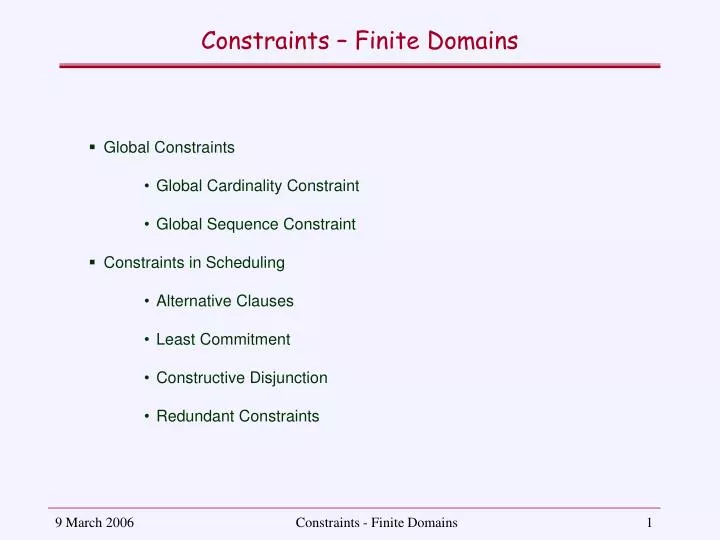
Constraints – Finite Domains. Global Constraints Global Cardinality Constraint Global Sequence Constraint Constraints in Scheduling Alternative Clauses Least Commitment Constructive Disjunction Redundant Constraints. Global Cardinality.

E N D
Constraints – Finite Domains • Global Constraints • Global Cardinality Constraint • Global Sequence Constraint • Constraints in Scheduling • Alternative Clauses • Least Commitment • Constructive Disjunction • Redundant Constraints Constraints - Finite Domains
Global Cardinality • Many scheduling and timetabling problems, have quantitative requirements of the type in these N “slots” M must be of type T • This type of constraints may be formulated with a cardinality constraint. In some sistems, these cardinality constraints are given as built-in, or may be implemented through reified constraints. • In particular, in SICStus the built-in constraint count/4 may be used to “count” elements in a list, which replaces some uses of the cardinality constraints (see ahead). • However, cardinality may be more efficiently propagated if considered globally. Constraints - Finite Domains
Global Cardinality • For example, assume a team of 7 people (nurses) where one or two must be assigned the morning shift (m), one or two the afternoon shift (a), one the night shift (n), while the others may be on holliday (h) or stay in reserve (r). • To model this problems, let us consider a list L, whose variables Li corresponding to the 7 people available, may take values in domain {m, a, n, h, r} (or {1, 2, 3, 4, 5} in languages like SICSTus that require domains to range over integers). • Both in SICStus or in CHIP this complex constraint may be decomposed in several cardinality constraints. Constraints - Finite Domains
Global Cardinality SICStus: count(1,L,#>=,1), count(1,L,#=<,2) % 1 or 2 m/1 count(2,L,#>=,1), count(2,L,#=<,2) % 1 or 2 a/2 count(3,L,#=, 1) , % 1 only n/3 count(4,L,#>=,0), count(4,L,#=<,2) % 0 to 2 h/4 count(5,L,#>=,0), count(5,L,#=<,2) % 0 to 2 r/5 CHIP: among([1,2],L,_,[1]), % 1 or 2 m/1 among([1,2],L,_,[2]), % 1 or 2 a/2 among( 1 ,L,_,[3]), % 1 only n/3 among([0,2],L,_,[4]), % 0 to 2 h/4 among([0,2],L,_,[5]), % 0 to 2 r/5 Constraints - Finite Domains
A m (1,2) B a (1,2) C n (1,1) D h (0,2) E r (0,2) F G Global Cardinality • Nevertheless, the separate, or local, handling of each of these constraints, does not detect all the pruning opportunities for the variables domains. Take the following example: A,B,C,D::{m,a}, E::{m,a,n}, F::{a,n,h,r}, G ::{n,r} Constraints - Finite Domains
A A m (1,2) B m (1,2) B a (1,2) C a(1,2) C n (1,1) D n (1,1) D h (0,2) E h (0,2) E r (0,2) F r (0,2) F G G Global Cardinality • A, B, C and D may only take values m and a. Since these may only be attributed to 4 people, no one else, namely E or F, may take these values m and a. • Since E may now only take value n, that must be taken by a single person, no one else (e.g. F or G) may take value n. Constraints - Finite Domains
Global Cardinality Constraint • This filtering, that could not be found in each constraint alone, can be obtained with an algorithm that uses analogy with results in maximum network flows [Regi96]. • A global cardinality constraint gcc/4, • constrains a list of k variables X = [X1, ..., Xk] , • taking values in the domain (with m values) V = [v1, ..., vm], • such that each of the vivalues must be assigned to between Li and Mivariables. • Then, m SICStus constraints ... count(vi,X,#>=,Li), count(vi,X,#=<,Mi) ... may be replaced by constraint gcc([X1....,Xk],[v1,...,vm],[L1,...,Lm],[M1,...,Mm]) Constraints - Finite Domains
A 0; 1 m (1,2) B 0; 1 t (1,2) C 1; 2 1; 2 n (1,1) D b 1 ; 1 a f (0,2) E 0; 2 0; 2 r (0,2) F G 0; Global Cardinality Constraint • The constraint gcc is modelled based on a parallel with a directed graph (or network) with maximum and minimum capacities in the arcs and two additional nodes, a e b. For example: gcc([A,,...,G],[m,t,n,f,r],[1,1,1,0,0],[2,2,1,2,2]) Constraints - Finite Domains
A 0; 1 m (1,2) B 0; 1 t (1,2) C 1; 2 1; 2 n (1,1) D b 1 ; 1 a f (0,2) E 0; 2 0; 2 r (0,2) F G 0; Global Cardinality Constraint • The constraint gcc is modelled based on a parallel with a directed graph (or network) with maximum and minimum capacities in the arcs and two additional nodes, a e b. For example: gcc([A,,...,G],[m,t,n,f,r],[1,1,1,0,0],[2,2,1,2,2]) Constraints - Finite Domains
A 0; 1 m (1,2) B 0; 1 t (1,2) C 1; 2 1; 2 n (1,1) D b 1 ; 1 a f (0,2) E 0; 2 0; 2 r (0,2) F G 0; Global Cardinality Constraint • A solution for the gcc constraint, corresponds to a flow between the two added nodes, with a unitary flow in the arcs that link variables to value nodes. In these conditions it is valid the following Theorem:A gcc constraint with k variables is satisfiable iff there is a maximal flow of value k, between nodes a and b Constraints - Finite Domains
Global Cardinality Constraint Of course, being gcc a global constraint it is intended to • Obtain a maximum flow with value k, i.e. to show whether the problem is satisfiable. • Achieve generalised arc consistency, by eliminating the arcs between variables that are not used in any maximum flow solution, i.e. do not belong to any gcc solution. • When some arcs are pruned (by other constraints) redo 1 and 2 incrementally. In [Regi96] a solution is presented for these problems, together with a study on its polinomial complexity. Constraints - Finite Domains
Global Cardinality Constraint 1. Obtain a maximal flow of value k • This optimisation problem may be efficiently solved by linear programming, that guarantees integer values in the solutions for the flows. • However, to take into account the intended incrementality, the maximal flow may be obtained by using increasing paths in the residual graph, until no increase is possible. • The residual graph of some flow f is again a directed graph, with the same nodes of the initial graph. Its arcs, with lower limit 0, have a residual capacity that accounts for the non used capacity in a flow f. Constraints - Finite Domains
Global Cardinality Constraint Residual graph of some flow f a. Given arc (a,b) with max capacity c(a,b) and flow f(a,b) such that f(a,b) < c(a,b) there is an arc (a,b) in the residual graph with residual capacity cr(a,b) = c(a,b) - f(a,b). The fact that the arc directions are the same means that the flow may still increase in that direction by up to value cr(a,b). b. Given arc (a,b) with min capacity l(a,b) and flow f(a,b) such that f(a,b) > l(a,b) there is an arc (b,a) in the residual graph with residual capacity cr(b,a) = f(a,b) - l(a,b). The fact that the arc directions are opposed means that the flow may decrease the initial flow by up to value cr(b,a). Constraints - Finite Domains
2 2 2 2 2 2 1 2 0 2 2 6 6 Global Cardinality Constraint Example: Given the following flow, with value 6 (lower than the maximal flow, which is of course 7) the following residual graph is obtained Constraints - Finite Domains
2 2 2 2 2 2 1 2 0 2 2 6 1 7 Global Cardinality Constraint • Existing an arc (a,b) (in the residual graph) whose flow is not the same as cr, there might be an overall increase in the flow between arcs a and b, if the arc belongs to an increasing path of the residual graph. • In the example below, the path in blue, increases the flow in the original graph up to its maximum. Constraints - Finite Domains
2 2 1 2 2 2 1 0 2 2 5 6 1 Global Cardinality Constraint • The computation of a maximal flow by this method is guaranteed by the following Theorem: A flow f between two nodes is maximal iff there is no increasing path for f between the nodes. • A decreasing path between a and b, could be defined similarly as a path in the residual graph between b and a shown below. Constraints - Finite Domains
Global Cardinality Constraint Complexity • The search for an increasing path may be obtained by a breadth-first search with complexity O(k+d+), where is the number of arcs between the nodes and their domains, with size d. As kd this is the dominant term, and the complexity is O(). • To obtain a maximum flow k, it is required to obtain k increasing paths, one for each of the k variables. The complexity of the method is thus O(k). • As kd, the complexity to obtain a maximal flow k, starting from a null flow is thus O(k2d). It is of course less, if the starting flow is not null. Constraints - Finite Domains
Global Cardinality Constraint • To eliminate arcs that correspond to assignments that do not belong to any possible solution, we use the following Theorem: Let f be a maximum flow between nodes, a and b. For any other nodes x and y, flow f(x,y) is equal to any flow f´(x,y) induced between these nodes by another maximal flow f’,iff the arcs (x,y) and (y,x)are not included in a cycle with more than 3 nodes that does not include nodes a and b. • Since the cycles considered do not include both a and b they will not change the (maximal) flow. Hence, if there are no cycles including nodes x and y, there are no increasing or decreasing paths through them that do not change the maximum flow. But then their flow will remain the same for all maximal flows. Constraints - Finite Domains
2 2 2 2 2 2 1 2 0 2 2 7 7 Global Cardinality Constraint Given the correspondence between maximal flow and the gcc constraint, if no maximum flow passes in an arc betwen a variable node X and a value node v, then for no solution of the gcc constraint is X = v. This can be illustrated in the maximal graph shown below. Constraints - Finite Domains
2 2 2 2 2 2 7 Global Cardinality Constraint • In the residual graph, the only paths with more than 3 nodes that do not include nodes a and b, are those shown at the right. Also shown, in blue, are the arcs with non null flow in the initial situation. These are all the arcs between variable and value nodes in a maximal flow, corresponding to possible solutions of constraint gcc/4. Constraints - Finite Domains
A m (1,2) B a (1,2) C n (1,1) D 2 h (0,2) E r (0,2) F G Global Cardinality Constraint • We may compare the initial graph with that obtained after the elimination of the arcs. • As expected, the latter fixes value n for variable E, and removes values m, a and n from variables F and G. Constraints - Finite Domains
Global Cardinality Constraint Complexity • Obtaining cycles with more than 3 nodes corresponds to obtain the subgraphs strongly connected, which can be done in O(m+n) for a graph with m nodes and n arcs. Here, m = k+d+1 and n kd+d, hence a global complexity of O(kd+2d+k+1) O(kd) • When some constraint removes a value from a variable that was included in the current maximal flow, a new maximal flow may have to be recomputed, with complexity at most O(k2d), so the complexity of using this incremental implementation of the gcc/4 constraint is O(k2d+kd) O(k2d). Constraints - Finite Domains
Global Cardinality Constraint • Recently [BoPA01] a global constraint was proposed to model and solve many network flow situations appearing in several problems, namely transport, communication or production chain applications. • As the previous ones, the goal of this constraint is to be integrated with other constraints, as a part of a more general problem, but allowing the efficient filtering that would not be possible if the constraint were decomposed into simpler ones. • Its use is described for problems of maximal flows, production planning and roastering. Constraints - Finite Domains
cars option capacity 1 2 3 4 5 6 7 8 9 10 1 1 / 2 X X X 2 2 / 3 X X X 3 1 / 3 X X 4 2 / 5 X X X 5 1 / 5 X Configuration 1 2 3 4 5 6 Global Constraint: Sequence Example (Car sequencing): The goal is to manufacture in an assembly line 10 cars with different options (1 to 5) shown in the table. Given the assembly conditions of option i, for each sequence of ni cars, only mi cars can have that option installed as shown in the table below. For example, in any sequence of 5 cars, only 2 may have option 4. instaled. Constraints - Finite Domains
Global Constraint: Sequence • Hence, the goal is to implement an efficient global sequence constraint , gsc/7 gsc(X, V, Seq, Lo, Up, Min, Max) with the following semantics: Given a sequence of variables X, Min and Max represent the minimum/maximumnumber of times they may take values from list V. Additionally, in each sequence of Seq variables, Lo and Up represent the minimum/maximum number of times they may take values from the listV. • Notice that in CHIP the gsc/7 constraints has a different syntax among([Seq, Lo, Up, Min, Max ], X, _, V) Constraints - Finite Domains
cars option capacity 1 2 3 4 5 6 7 8 9 10 1 1 / 2 X X X 2 2 / 3 X X X 3 1 / 3 X X 4 2 / 5 X X X 5 1 / 5 X Configuration 1 2 3 4 5 6 Global Constraint: Sequence • The following program specifies the sequencing constraints of this problem goal(X):- X = [X1, .. ,X10], L :: 1..6, gcc(X, L, [1,1,2,2,2,2], [1,1,2,2,2,2]), % gsc(X, V, Seq, Lo, Up, Min, Max) gsc(X, [1,5,6], 2, 1, 1, 5, 5), % option 1 gsc(X, [3,4,6], 3, 2, 2, 6, 6), % option 2 gsc(X, [1,5] , 3, 1, 1, 3, 3), % option 3 gsc(X, [1,2,4], 5, 2, 2, 4, 4), % option 4 gsc(X, [3] , 5, 1, 1, 2, 2). % option 5 Constraints - Finite Domains
Global Constraint: Sequence • Given the similarity of the constraints, it was proposed in [RePu97] an efficient implementation of the global sequencing constraint, gsc/7, based on the global cardinality constraint, gcc/4. • The way this implementation takes place can be explained by means of an example. • Given sequence X = [X1 .. X15], with X :: 1..4, it is intended that values [1,2] appear between 8 and 12 times, and that each sequence of 7 variables contains these values between 4 and 5 times , i.e. gsc(X, [1,2], 7, 4, 5, 8, 12) Constraints - Finite Domains
Global Constraint: Sequence gsc(X, [1,2], 7, 4, 5, 8, 12) • We may begin with, by considering a new set of variables Ai, distributed in subsequences S1, S2and S3 of 7 elements each (except the last). The values of each Ak that belong to sequence Skare defined as Xi [1,2] Ai = v , Xi [1,2] Ai = ak • Clearly, there might not exist less than 2 nor more than 3 values a1and a2in the whole sequence A, to guarantee between 4 and 5 values [1,2]in S1 and S2 Constraints - Finite Domains
Global Constraint: Sequence gsc(X, [1,2], 7 , 4, 5, 8, 12) gsc(X, V , Seq , Lo, Up, Max, Min) • One must still guarantee the existence of between 8 (Min) and 12 (Max) vs in the Ai sequences. • All these conditions are met, with the constraints that map the Xis into Ais, and also with the global cardinality constraint gcc(A, [v,a1,a2,a3], [8,2,2,0], [12,3,3,1]) Constraints - Finite Domains
Global Constraint: Sequence • Not all sequences of 7(Seq) elements were already considered. For thus purpose, 7 (Seq) gcc constraints must be considerd as shown in the figure • All these conditions are met, with the constraints that map the Xis into Ais, and also with the global cardinality constraint gcc(A, [v,a1,a2,a3], [8,2,2,0], [12,3,3,1]) Constraints - Finite Domains
Global Constraint: Sequence The gsc constraint is thus mapped into 7 gcc constraints gcc(A, [v,a1,a2,a3], [8,2,2,0], [12,3,3,1]) gcc(B, [v,b1,b2,b3], [8,0,2,2], [12,1,3,3]) gcc(C, [v,c1,c2,c3], [8,0,2,1], [12,2,3,3]) gcc(D, [v,d1,d2,d3], [8,0,2,2], [12,3,3,3]) gcc(E, [v,e1,e2,e3], [8,0,2,0], [12,3,3,3]) gcc(F, [v,f1,f2,f3], [8,0,2,0], [12,3,3,3]) gcc(G, [v,g1,g2,g3], [8,1,2,0], [12,3,3,2]) gcc(A, [v,a1,a2,a3], [8,2,2,0], [12,3,3,1]) Constraints - Finite Domains
Scheduling Problems • In addition to global sequencing constraints, there are other important constraints in a variety of scheduling problems (job-shop, timetabling, roastering, etc...). Some important constraints are • Precedence : one task executes before the other • Non-overlapping: Two tasks should not execute at the same time (e.g. they share the same resource). • Cumulation: The number of tasks that execute at the same time must not exceed a certain number (e.g. the number of resources, such as machines or people, that must be dedicated to one of these tasks). Constraints - Finite Domains
Precedence • In general, each task i is modeled by its starting time Ti and its duration Di, which may both be either finite domain variables or fixed to constant values. Hence, the precedence of task i with respect to task j may be expressed simply as before(Ti, Di, Tj) :- Ti + Di #=< Tj. • In practice, such specification of precedence is equivalent to the following specification with indexical constraints, by means of fd_predicates. For example, before(Ti, Di, Tj)+: Ti in inf .. max(Tj)-min(Di) Di in inf .. max(Tj)-min(Ti) Tj in min(Ti)+min(Di) .. Sup which implements bounds consistency. Constraints - Finite Domains
Non Overlapping • The non overlapping of tasks is equivalent to the disjunction of two precedence constraints: • Either • Task i executes before Task j; or • Task j executes before Task i. • Many different possibilities exist to implement this disjunction, namely, by means of: • Alternative clauses; • Least commitement; • Constructive Disjunction • Specialised global constraints Constraints - Finite Domains
T1/2 T2/4 T3/3 T4/1 Non Overlapping Example Let us consider a project with the four tasks illustrated in the graph, showing precedences between them, as well as mutual exclusion (). The durations are shown in the nodes. The goal is to schedule the taks so that T4 ends no later than time 10. (see program tasks) project(T):- domain([T1,T2,T3,T4], 1, 10), before(T1, 2, T2), before(T1, 2, T3), before(T2, 4, T4), before(T3, 3, T4), no_overlap(T2, 4, T3, 3). Constraints - Finite Domains
Non Overlapping Alternative clauses • In a Constraint Logic Programming system, the disjunction of constraint may be implemented with a Logic Programming style (a la Prolog): no_overlap(T1, D1, T2, _):- before(T1, D1, T2). no_overlap(T1, _, T2, D2):- before(T2, D2, T1). This implementation always tries first to schedule task T1 before T2, and this may be either impossible or undesirable in a global context. This greatest commitment will usually show poor efficiency (namely in large and complex problems). Constraints - Finite Domains
Non Overlapping Least Commitment • The opposite least commitment implementation may be made through the cardinality constraint no_overlap(T1,D1,T2,D2):- card(1, 1, [T1 + D1 #=< T2, T2 + D2 #=< T1]). or directly, with propositional constraints no_overlap(T1,D1,T2,D2):- (T1 + D1 #=< T2) #\ (T2 + D2 #=< T1). or even with reified constraints no_overlap(T1,D1,T2,D2):- (T1 + D1 #=< T2) #<=> B1, (T2 + D2 #=< T1) #<=> B2, B1 + B2 #= 1. • When enumeration starts, if eventually one of the constraints is disentailed, the other is enforced. Constraints - Finite Domains
Non Overlapping Constructive Disjunction • With constructive disjunction, the values that are not part of any solution may be removed, even before a commitment is mode regarding which of the tasks is executed first. Its implementation may be done directly with the appropriate indexical constraints. • For example, the constraint T1 + D1 #=< T2 can be compiled into T1 in inf..max(T2)-min(D1), T2 in min(T1)+min(D1)..sup, D1 in inf..max(T2)-min(T1) Constraints - Finite Domains
Non Overlapping Constructive Disjunction • Compiling similarly the other constraint we have either or that can be combined together as no_overlap3(T1, D1, T2, D2)+: T1 in inf..max(T2)- min(D1))\/ min(T2)+min(D2)..sup), T2 in inf..max(T1)- min(D2))\/ min(T1)+min(D1)..sup), D1 in (inf..max(T2)-min(T1))\/ (min(D1) .. max(D1)), D2 in (inf..max(T1)-min(T2))\/ (min(D2) .. max(D2)). T2 in inf..max(T1)-min(D2), T1 in min(T2)+min(D2)..sup, D2 in inf..max(T1)-min(T2) T1 in inf..max(T2)-min(D1), T2 in min(T1)+min(D1)..sup, D1 in inf..max(T2)-min(T1) Constraints - Finite Domains
Non Overlapping Global Constraint serialized/3 • In this problem, the 4 tasks end up being executed with no overlaping at all. For this situation, global constraint serialized/3 may be used. • This global constraint serialized(T,D,O) contrains the tasks whose start times are input in list T, and the durations are input in list D to be serialised, i.e. to be executed with no overlapping. O is a (possibly empty) list with some options available for the execution of the constraint, that allow different degrees of filtering. • As usual, the more filtering power is required, the more time serialized/3 takes to execute Constraints - Finite Domains
Non Overlapping Global Constraint serialized/3 • Given this built-in global constraint we may express the non overlap requirement directly as no_overlap([T1,T2,T3,T4],[2,4,3,1]):- serialized([T1, T2,T3,T4],[2,4,3,1], [edge_finder(true)]) Notice the use of option edge_finder, that implements an algorithm, based on [CaPi94], to optimise the detection of the edges (beginnings and ends) of the tasks under consideration. Constraints - Finite Domains
Non Overlapping Results: Alternative Clauses • With alternative clauses, the solutions are computed in alternative. Notice that since some ordering of the tasks is imposed, the domains of the variables are highly constrained in each alternative. |? T in 1..10, project(T). T1 = 1 ,T2 = 3, T3 = 7, T4 = 10 ? ; T1 = 1 ,T2 = 6, T3 = 3, T4 = 10 ? ; no |? T in 1..11, project(T). T1 in 1..2, T2 in 3..4, T3 in 7..8, T4 in 10..11 ? ; T1 in 1..2, T2 in 6..7, T3 in 3..4, T4 in 10..11 ? ; no Constraints - Finite Domains
Non Overlapping Results: Least Commitment • With the least commitment, little prunning is achieved. Before enumeration, and because the system is not able to “reason” globally with the non_overlap and the precedence consraints, it only considers separately sequences T1, T2 and T4 as well as T1, T3 e T4, and hence the less significative prunning of the end of T1 and the begining of T4. |? T in 1..10, project(T). T1 in 1 .. 4, T2 in 3 .. 6, T3 in 3 .. 7, T4 in 7 .. 10 ? ; no |? T in 1..11, project(T). T1 in 1 .. 5, T2 in 3 .. 7, T3 in 3 .. 8, T4 in 7 .. 11 ? ; no Constraints - Finite Domains
Non Overlapping Results: Constructive Disjunction • With the constructive disjunction formulation, the same cuts are obtained in T1 and T4 (again there is no global reasoning). However, the constructive disjunction does prune values of T2 e T3, by considering the two possible sequences of them. |? T in 1..10, project(T). T1 in 1 .. 4, T2 in{3} \/ {6}, T3 in{3} \/ {7}, T4 in 7.. 10 ? ; no |? T in 1..11, project(T). T1 in 1 .. 5, T2 in(3..4) \/ (6..7), T3 in(3..4) \/ (7..8), T4 in 7 .. 11 ? ; no Constraints - Finite Domains
Non Overlapping Results: Serialised With the serialized constraint (with the edgefinder option on), not only is the system able to restrict the values of T2 and T3, but it also detects that T2 and T3 are both, in any order, between T1 and T4 which helps pruning the starting time of T1 (but not of T4, in the second case). |? T in 1..10, project(T). T1 = 1, T2 in{3} \/ {6}, T3 in{3} \/ {7}, T4 = 10 ? ; no |? T in 1..11, project(T). T1 in 1 .. 2, T2 in(3..4) \/ (6..7), T3 in(3..4) \/ (7..8), T4 in 7 .. 11 ? ; no Constraints - Finite Domains
Redundant Constraints Redundancy • Not even the specification with a global serialised constraint was able to infer all the prunnings that should have been made. • This is of course a common situation, as the constraint solvers are incomplete. • In many situations it is possible to formulate constraints which can be deduced from the initial ones, i.e. that should not make any difference in the set of results obtained. • However, if properly thought of, they may provide a precious support to the constraint solver, enabling a degree of pruning that the solver would not be able to make otherwise . Constraints - Finite Domains
Redundant Constraints Redundancy • Hence the name of redundant constraints.Careful use of such constraints may greatly help to increase the efficiency of constraint solving. • Of course, is up to the user to understand the working of the solver, and its pitfalls, in order to formulate adequate redundant constraints. • In this case, tasks 2 and 3 may never terminate before total duration of both is added to the starting time of the first of them. • Hence, task T4 may never start before min(min(T2),min(T3))+D2+D3 Constraints - Finite Domains
Redundant Constraints Specifying Redundancy In SICStus, such redundant constraint can be expressed as follows. • First an interval is created during which T4 (in general, all the tasks that must be anteceded by both T2 and T3) must start execution. This interval is not upper bounded but its lower bound is min(min(T2),min(T3))+D2+D3 Such interval can be created as the union of two intervals by means of the indexical expression (min(T2)+D2+D3..sup)\/(min(T3)+D2+D3..sup)) Constraints - Finite Domains
Redundant Constraints Specifying Redundancy • Now it must be guaranteed that task T4 executes within this interval. This may be achieved in many ways. One possibility is to assume that the interval just considered is the start time of a task Edge23_up, with null duration, that must be executed before task T4, i.e. Edge23_up in (min(T2)+D2+D3..sup)\/(min(T3)+D2+D3..sup)) • With the previous predicates, the precedence of this dummy task with respect to T4 is specified simply as before(Edge23_up, 0, T4) Constraints - Finite Domains
Redundant Constraints Specifying Redundancy • The same reasoning may now be used to define the time, by which must end all the tasks (in this case T1) that execute before both tasks T2 and T3. This end must occur no later than max(max(T2+D2),max(T3+D3)-D2-D3) ... which simplifies to max(max(T2-D3),max(T3-D2)) This can thus be the ending time of a task with null duration Edge23_lo, which can be specified again as the union of two intervals Edge23_lo in (inf .. max(T2)-D3)\/( inf .. max(T3)-D2) Constraints - Finite Domains