Download
1 / 35
370 likes | 544 Views
Quantum Optics with single Nano-Objects. Outline:. Introduction : nonlinear optics with single molecule Single Photon sources Photon antibunching in single quantum dot fluorescence Conclusion. A D VANTAGES. No ensemble averaging Statistical correlations

E N D
Outline: • Introduction : nonlinear optics with single molecule • Single Photon sources • Photon antibunching in single quantum dot fluorescence • Conclusion
ADVANTAGES • No ensemble averaging • Statistical correlations • Extreme sensitivity to immediate local nanoenvironment • No synchronisation needed, time evolution • Single quantum system
Fluorescence Laser detuning (MHz) Inhomogenous spectrum at 2 K l = 620 nm Fluorescence Laser detuning (GHz) Saturation of a SM line ghom= 20 MHz I ~ 250Is
wp ws ws w0 wp wp - Light Shift - Hyper-Raman Resonance Pump-probe experiments: Fluorescence (a. u.) Pump-Probe Detuning (MHz)
W = 2.4 G W = 4.7 G Light shift (G) Inverse pump detuning (G-1)
Linear Stark Shift: Dm ~ 0.3 D Electro-Optical Effects E0RF cos(wRF t) Linear Coupling with the RF field - 1st case: High RF field, low laser intensity Modulation of the molecular transition frequency Side Bands Modulation of the laser frequency
wRF = 80 MHz x = 0 x = 2.5 x = 5
|1,n> |e,n> dL WL |g,n+1> |2,n> 2nd case: High laser intensity, low RF field • Molecule dressed • by the laser field • RF coupling between 1,n> and |2,n> states - Rabi Resonance: wRF = WG fixed wRF, tuneddL dL 0
Shift of the Rabiresonance function of the laser field amplitude WL=3.5G WL=1.5G
Quantum Cryptography: * Quantum mechanics provide unconditional security for communication * Encoding information on the polarization of single photons Quantum computing: Quantum logic gates based on single photons have been demonstrated Triggered Single Photon Sources Practical need for Single Photons:
Present day sources of single photons • - Correlated photon pairs • * Atomic cascade • * Parametric down conversion • - Highly attenuated laser (or LED) pulses • Problems: • Random time generation • Average photon’s number <<1 Present day sources of single photons
Use of a single quantum system • Yamamoto’s group experiment: • - Coulomb Blockade in a mesoscopic double barrier p-n junction • temperature 50 mK (dilution cryostat) • low detection efficiency ~10-4 • low e-h recombination rate
Photon antibunching in single molecule fluorescence Deterministic generation of single photons Controlled excitation of a single molecule
|g,n+1> |1,n> |e,n> |e,n> |2,n> |g,n> |g,n+1> |1,n-1> |e,n-1> |e,n-1> |2,n-1> |g,n-1> |g,n> |1,n-2> |e,n-2> |e,n-2> |2,n-2> |g,n-1> -d0 +d0 0 Excitation: Rapid adiabatic passage Two conditions: Adiabatic passage Tpass > TRabi Rapid passage Tpass << tf WL >> G
+30 +45 0 0 Voltage (V) Detuning (G) -30 -45 Fluorescence Time (ns) nRF = 3 MHz, WL = 2.6 G
Detailed shape of a fluorescence burst - T = 250 ns, = 3 , 0 = 80 - Short rise time - Relaxation time (-1 8 ns) - Oscillations
How many emitted photons per sweep? Measurement of the autocorrelation function g(2)(t) Comparaison with Q.M.C. simulations
d0 = 25G 1200 4 800 2 400 0 d0 = 44G 6 800 4 Number of Coincidences Correlation Function (u. a.) 2 400 0 d0 = 65G 600 400 -200 0 200 -200 0 200 Delay (ns) Histogram of time delays: nRF = 3MHz, WL = 3.2 G 6 4 2 0
Comparaison with a Coherent source - n = 6 MHz, d0 = 44G - nav = 1.12 • p(1) = 0.68 - p(n>1) ~ 0.21 - Mandel Parameter Q sour.= - 0.65 Qdetc.= - 0.006
Start Excitation (532nm) T.A.C. & P.H.A. Fluorescence Stop Room Temperature Single photon source • Principe de l’expérience • Pulsed excitation to a vibrationnaly excite level • Rapid Relaxation (ps) to the fluorescent state • Emission of a single photon • Experimental setup • - Inverted Microscope • - Piezo-electric Scanner • Coincidence Setup • Detection effeciency 6%
System:Terrylene in p-terphenyl Favorable photophysical parameters and high photostability Confocal fluorescence image(10mm*10mm) of single Terrylene molecules
1600 mW 670 mW 210 mW 50mW 20 mW CW Excitation : Photon Antibunching Fluorescence autocorrelation function g(2)(t) proportional to the excited state population, t>0: Signature of a single molecule emission
Pulsed excitation : Triggered single photon emission - M.L. 532 nm laser: - Pulse width: 35ps, - Repetition rate: n = 6.25 MHz • Single exponential decay • - fluorescence lifetime: • tf = 3.8 ns
Fluorescence autocorrelation Function • Laser spot positioned • on a single molecule (Signal/Background~ 6) • (b) Away from any molecule (background coherent emission ) central peak area / lateral peak area = (B2+2BS) / (B+S)2 ~ 0.27
Saturation du taux d’émission Short laser pulse : tp<<tf p(2) ~ 0 p(1) =P(t=tp) Emission rate: S= h np(1)= S P(tp) At the maximum power : Smax=310 kHz, pmax(1)=0.86 Fit: S=343 kHz, Is=1.2 MW/cm2 86% of the pulses lead to a single photon emission
Comparaison with a coherent source - nav = 0.86 - p(1) = 0.86 - n = 6.25 MHz - Mandel Parameter Q sour.= - 0.86 Qdetc.= - 0.03 - P(n>1) < 8 10-4 !
ZnS CdSe Photon statistics of single quantum dot fluorescence • - QDs bridge the gap between • single molecules and bulk solid state • Size-dependent optical properties • - Tunable absorbers and emitters • - Applications from labeling to nano-devices • Colloidal CdSe/ZnS quantum dots • 2 nm Radius, 575 peak emission • fluorescence quantum yield ~50%, e ~ 105 M-1 cm-1
Intermittence in single QD Fluorescence - High S/B ratio - Low photobleaching rate fblea < 10-8 Blinking: ton , Intensity dependence toff , no I dependence, inverse power law - Blinking attributed to Auger ionization
Photon antibunching in single QD fluorescence • Start-Stop setup • Coincidence histogram C(t) • (TAC time window tTAC of200 ns, bin width tbin of 0.2 ns) Dip at t=0, signature of a strong photon antibunching C(0) ~ 0 for a large range of intensities (0.1 – 100 kW/cm2) High Auger ionization rates (~1/20 ps-1, Klimov et al.) No multi-excitonic radiative recombination
Quantum dot lifetimes measurements Single QDs measurements at low intensities • - Experimental accuracy ~ ns • Width of tf histogram : heterogenety in the QDs structure !? Bulk measurement with TCSPC (M. Dahan et al., 2000) Multi-exponential decay
From the QD state filling equations Saturation intensities: Isat ~ 10-80 kW/cm2 Cross-section : sabs ~ 2 – 16 10-16 cm2
Count rate saturation • At high intensities, very short ton , average count rate Rav skewed • Use coincidence histogram for accurate value Rav in the On state • With large tTAC and high Rav, t ~ interphoton mean time (1/ Rav) Good agreemeny For the measured Isat
Conclusion • Demonstration of a single photon source based on controlled fluorescence from single molecule • Room temperature operation - Improve the collection efficiency de collection (cavity…) • Other systems: * NV centers (antibunching observed) * Quantum dots : at low T (<5K) antibunching in spectrally selected fluorescence from InAs QDs • Photon antibunching in colloidal CdSe QDs Efficient Auger ionization effect