Download
1 / 34
340 likes | 429 Views
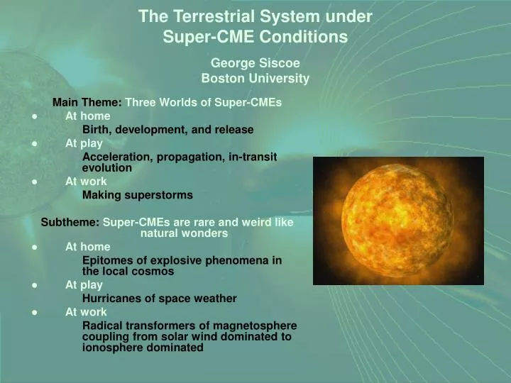
The Terrestrial System under Super-CME Conditions George Siscoe Boston University. Main Theme: Three Worlds of Super-CMEs At home Birth, development, and release At play Acceleration, propagation, in-transit evolution At work Making superstorms

E N D
The Terrestrial System under Super-CME ConditionsGeorge SiscoeBoston University Main Theme: Three Worlds of Super-CMEs • At home Birth, development, and release • At play Acceleration, propagation, in-transit evolution • At work Making superstorms Subtheme: Super-CMEs are rare and weird like natural wonders • At home Epitomes of explosive phenomena in the local cosmos • At play Hurricanes of space weather • At work Radical transformers of magnetosphere coupling from solar wind dominated to ionosphere dominated
Super-CMEs at HomeBirth, Development, and Release Composite H alpha Soft X-ray Continuum Magnetogram Relation to active region, prominences, and “sigmoids” Illustrated by event on November 4, 2001
upper separatrix lower separatrix Photospheric Field Topology of Titov & Démoulin 1999 Model upper separatrix lower separatrix upper separatrix
Relation to magnetic arcades Illustrated by Bastille Day event
Release Mechanisms Flux Cancellation Breakout Terry Forbes Spiro Antiochos
Observable Implication of CME Models (Crooker, 2005) • FLUX-CANCELLATION MODEL • Dipolar fields reconnect • Leading field matches dipolar component • BREAKOUT MODEL • Quadrupolar fields reconnect • Leading field opposes dipolar component • Taken at face value, imprint of dipolar component on leading field and leg polarity favors streamer over breakout model by ~80%.
Super-CMEs at PlayAcceleration, propagation, in-transit evolution 1500 Jie Zhang data 1250 1000 750 500 250 50 100 150 200
Inflationary Phase Geometrical Dilation + Radial Expansion Phase Sun CME Pre-CME Growth Phase Three Phases of CME Expansion MHD simulation Pete Riley
1400 1200 1000 800 600 400 200 50 100 150 200 drag Cd ρ (V-Vsw)2 Standard Form Observed Information on Interplanetary CME Propagation Gopalswamy et al., GRL 2000: statistical analysis of CME deceleration between ~15 Rs and 1 AU Reiner et al. Solar Wind 10 2003: constraint on form of drag term in equation of motion
Accelerate 80 Vexp = 0.266 Vcme – 71.61 60 Decelerate 40 20 350 400 450 500 550 600 Information on CME Parameters at 1 AU Vršnak and Gopalswamy, JGR 2002: velocity range at 1 AU << than at ~ 15 Rs Owen et al. 2004: expansion speed CME speed; B field uncorrelated with speed; typical size ~ 40 Rs Lepping et al, Solar Physics, 2003: Average density ~ 11/cm2; average B ~ 13 nT
Gopalswamy et al. MHD Simulation 1000 Analytical No Virtual Mass 800 400 Circular CME Velocity (km/s) Variable CD 600 Virtual Mass 300 400 Fixed CD Velocity (km/s) Acceleration (m/s/s) 200 200 1400 1.5 2 2.5 3 3.5 4 4.5 5 1200 100 1000 Distance from the Sun (Rs) 800 10 20 30 40 50 drag Cd ρ (V-Vsw)2 Standard Form Distance from Sun (Rs) 600 Distance from Sun Center (Rs) 400 Observed 200 50 100 150 200 Analytical model of CME Acceleration and Propagation Generalized buoyancy Elliptical cross section Variable drag coefficient Satisfies Gopalswamy template Satisfies Reiner template Virtual mass Comparison with MHDsimulation
1500 1250 1000 750 500 250 from Crooker, 2004 50 100 150 200 Predictability (Crooker) • Cloud axis • Aligns with filament axis (low) and HCS (high) • Directed along dipolar field distorted by differential rotation • Leading field • Aligns with coronal dipolar field (high) • Application • First part predicts the rest (Chen et al., 1997) • Cloud axis orientation, Fair • 28/50 (56%) align within 30° of neutral line [Blanco et al., 2005] • Leading field, Good • 33/41 (80%) match solar dipolar component with 2-3 year lag [Bothmer and Rust, 1997] • 28/38 (74%) from PVO match [Mulligan et al., 1998]
1500 1250 1000 750 1400 500 1200 1000 250 800 600 400 50 100 150 200 200 50 100 150 200 CME Propagation Models Gopalswamy Template • Empirical model of CME deceleration (Gopalswamy et al., 2000) • Analytical model of CME propagation (Siscoe, 2004) • Numerical simulation 0.5 to 50 AU (Odstrcil et al., 2001) • Numerical simulation 1 Rs to 1 AU with two codes (Odstrcil et al., 2002)
Solar Wind Dominated Ionosphere Dominated Dynamic Pressure (nPa) Super-CMEs at Work Making Superstorms • Psw distributions in CIRs and CMEs (Lindsay et al., 1995) • Ey distributions in CIRs and CMEs (Lindsay et al., 1995) • GeoImpact of CMEs (Gosling, 1990)
The Terrestrial System under Super-CME Conditions • Vasyliunas Dichotomization Solar wind dominated Ionosphere dominated • Solar wind dominated Global force balance via Chapman-Ferraro current system Dst responds to ram pressure • Ionosphere dominated Global force balance via region 1 current system Neutral flywheel effect No (direct) Dst response to ram pressure Magnetopause erosion • Transpolar potential saturation (TPS) Equivalent to ionosphere dominated regime Evidence for TPS and the Hill model parameterization
Vasyliunas Dichotomization Vasyliunas (2004) divided magnetospheres into solar wind dominated and ionosphere dominated depending on whether the magnetic pressure generated by the reconnection-driven ionospheric current is, respectively, less than or greater than the solar wind ram pressure. The operative criterion is • oPVAε ~ 1 • P = ionospheric Pedersen conductance VA = Alfvén speed in the solar wind ε = magnetic reconnection efficiency Key Point By this criterion, the standard magnetosphere is solar wind dominated; the storm-time magnetosphere, ionosphere dominated.
Chapman & Ferraro, 1931 Midgley & Davis, 1963 z C-F compression = 2.3 dipole field 2x10⁷ N x Pertinent Properties of the Standard Magnetosphere Chapman-Ferraro Current System ICF = BSS Zn.p./o 3.5 MA
GOES 8 April 2000 storm Huttunen et al., 2002 Ram Pressure Contribution to Dst A Chapman-Ferraro property Psw compresses the magnetosphere and Increases the magnetic field on the dayside. Chapman-Ferraro Compression
V E B 500 400 300 Transpolar Potential (kV) 200 100 5 10 15 20 Ey (mV/m) Interplanetary Electric Field Determines Transpolar Potential A magnetopause reconnection property • Magnetopause reconnection • Equals transpolar potential • Transpolar potential varies linarly with Ey (Boyle et al., 1997) • Magnetosphere a voltage source as seen by ionosphere IMF = (0, 0, -5) nT
Solar Wind Dominated Magnetosphere Summary • Psw compresses the magnetospheric field and increases Dst. • Ey increases the transpolar potential linearly. • Magnetosphere a voltage source Key Point Field compression and linearity of response to Ey hold foronly one of the two modes of magnetospheric responsesto solar wind drivers—the usual one.
1 MA/10 Re 5.5 MA Iijima & Potemra, 1976 Region 1 Atkinson, 1978 Region 2 3.5 MA R 1 Tail C-F Total Field-Aligned Currents for Moderate Activity (IEF ~1 mV/m) Region 1 : 2 MA Region 2 : 1.5 MA Then Came Field-Aligned Currents Question: How do you self-consistently accommodate the extra 2 MA?
Answer: You Don’t. You replace the Chapman-Ferraro current with it. IMF = (0, 0, -5) nT
Region 1 Current Contours Region 1 Current Streamlines 5x10⁶ N Region 1 Force on Earth IMF = (0, 0, -5) nT
Impact of Region 1 Currents on Understanding Solar Wind-Magnetosphere Coupling Summary • Ionosphere and solar wind in “direct” contact • Solar wind can pull on ionosphere as well as push on earth. • Region 1 currents can usurp Chapman-Ferraro currents. • Influence of ionosphere coupling increases relative to Chapman-Ferraro coupling as interplanetary electric field (Ey) increases. Key Point During major magnetic storms, this leads to an ionosphere dominated magnetosphere
What does this mean? It means that whereas the standard magnetosphere interacts with the solar wind mainly by currents thatflow in and on the magnetosphere, the storm-time magnetosphere interacts with the region 1 current system that links the ionosphere to the solar wind in the magnetosheath and the bow shock.
Chapman- Ferraro Region 1 350 PSW=10 300 250 Baseline (PSW=1.67, Σ=6) 200 Transpolar Potential (kV) 150 Σ=12 100 50 57 . 6 E sw F = IMF = 0 IMF Bz = -30 H 1 6 / P 10 20 30 40 50 sw Ey (mV/m) Linear regime (small ESW) Saturation regime (big ESW) Transpolar Potential Saturation
Bow Shock Streamlines Region 1 Current Cusp Ram Pressure Reconnection Current And most important • Region 1 current gives the J in the JxB force that stands off the solar wind • And communicates the force to the ionosphere • Which communicates it to the neutral atmosphere as the flywheel effect Richmond et al., 2003
Cahill & Winckler, 1999 Dipole Field GOES 8 April 2000 storm Hairston et al., 2004 Huttunen et al., 2002 500 400 300 Transpolar Potential (kV) 200 100 5 10 15 20 Ey (mV/m) Evidence of Two Coupling Modes • Transpolar potential saturation Instead of this You have this • No dayside compression seen at synchronous orbit Instead of this You have this
Jordanova, 2005 b = 11.7 McPherron, 2004 Lee et al., 2004 To Resume • Transpolar potential saturation • No dayside compression seen at synchronous orbit • No compression term (b) in the Burton-McPherron-Russell equation: dDst*/dt = E – Dst*/ Dst* = Dst - b√Psw Instead of this You have this • Ring current model fits storm main phase better without pressure correction • Possibly related: Large parallel potential drops Sawtooth events
The Bimodal Magnetosphere Quiet Magnetosphere Dominant current system Chapman-Ferraro (Region 1 lesser) Magnetopause current closes on magnetopause Magnetopause a bullet-shaped quasi-tangential discontinuity Transpolar potential proportional to IEF Solar wind a voltage source for ionosphere Compression strengthens dayside magnetic field Minor magnetosphere erosion Main dynamical mode: substorms Force transfer by dipole Interaction Superstorm Magnetosphere Dominant current system Region 1 (no Chapman-Ferraro) Magnetopause current closes through ionosphere and bow shock Magnetopause a system of MHD waves with a dimple Transpolar potential saturates Solar wind a current source for ionosphere Stretching weakens dayside magnetic field Major magnetosphere erosion Main dynamical mode: storms Force transfer by ion drag Summary Dichotomization, transpolar potential saturation, no Dst response to ram pressure, magnetopause erosion, neutral flywheel effect all part of one story.
THE END Thank You
45o 5 nT 0o 5 nT Cahill & Winckler, 1999 Dipole Field 180o 30 nT 90o 5 nT 180o 20 nT 180o 2 nT 180o 10 nT You have this
Region 1 Current Contours Properties of Ionosphere-Dominated Magnetosphere Region 1 Current System Fills Magnetopause