Download
1 / 63
630 likes | 815 Views
Stanford CS223B Computer Vision, Winter 2006 Lecture 2 Lenses, Filters, Features. Professor Sebastian Thrun CAs: Dan Maynes-Aminzade and Mitul Saha [with slides by D Forsyth, D. Lowe, M. Polleyfeys, C. Rasmussen, G. Loy, D. Jacobs, J. Rehg, A, Hanson, G. Bradski,…] . Today’s Goals.

E N D
Stanford CS223B Computer Vision, Winter 2006Lecture 2 Lenses, Filters, Features Professor Sebastian Thrun CAs: Dan Maynes-Aminzade and Mitul Saha [with slides by D Forsyth, D. Lowe, M. Polleyfeys, C. Rasmussen, G. Loy, D. Jacobs, J. Rehg, A, Hanson, G. Bradski,…]
Today’s Goals • Thin Lens • Aberrations • Features 101 • Linear Filters and Edge Detection
Pinhole Camera (last Wednesday) -- Brunelleschi, XVth Century Marc Pollefeys comp256, Lect 2
Snell’s Law Snell’s law n1 sina1 = n2 sin a2
Thin Lens: Definition focus optical axis f Spherical lense surface: Parallel rays are refracted to single point
Thin Lens: Projection optical axis Image plane f z Spherical lense surface: Parallel rays are refracted to single point
Thin Lens: Projection optical axis Image plane f f z Spherical lense surface: Parallel rays are refracted to single point
Thin Lens: Properties • Any ray entering a thin lens parallel to the optical axis must go through the focus on other side • Any ray entering through the focus on one side will be parallel to the optical axis on the other side
Thin Lens: Model Q P O Fr Fl p R Z f f z
The Thin Lens Law Q P O Fr Fl p R Z f f z
Limits of the Thin Lens Model 3 assumptions : • all rays from a point are focused onto 1 image point • Remember thin lens small angle assumption 2. all image points in a single plane 3. magnification is constant Deviations from this ideal are aberrations
Today’s Goals • Thin Lens • Aberrations • Features 101 • Linear Filters and Edge Detection
Aberrations 2 types : geometrical : geometry of the lense, small for paraxial rays chromatic : refractive index function of wavelength Marc Pollefeys
Geometrical Aberrations • spherical aberration • astigmatism • distortion • coma aberrations are reduced by combining lenses
Astigmatism Different focal length for inclined rays Marc Pollefeys
Astigmatism Different focal length for inclined rays Marc Pollefeys
Spherical Aberration rays parallel to the axis do not converge outer portions of the lens yield smaller focal lenghts
Distortion magnification/focal length different for different angles of inclination pincushion (tele-photo) barrel (wide-angle) Can be corrected! (if parameters are know) Marc Pollefeys
Coma point off the axis depicted as comet shaped blob Marc Pollefeys
Chromatic Aberration rays of different wavelengths focused in different planes cannot be removed completely Marc Pollefeys
Vignetting Effect: Darkens pixels near the image boundary
CCD vs. CMOS Mature technology Specific technology High production cost High power consumption Higher fill rate Blooming Sequential readout Recent technology Standard IC technology Cheap Low power Less sensitive Per pixel amplification Random pixel access Smart pixels On chip integration with other components Marc Pollefeys
Today’s Goals • Thin Lens • Aberrations • Features 101 • Linear Filters and Edge Detection
Today’s Question • What is a feature? • What is an image filter? • How can we find corners? • How can we find edges? • (How can we find cars in images?)
What is a Feature? • Local, meaningful, detectable parts of the image
Features in Computer Vision • What is a feature? • Location of sudden change • Why use features? • Information content high • Invariant to change of view point, illumination • Reduces computational burden
(One Type of) Computer Vision Image 1 Image 2 Feature 1 Feature 2 : Feature N Feature 1 Feature 2 : Feature N Computer Vision Algorithm
Where Features Are Used • Calibration • Image Segmentation • Correspondence in multiple images (stereo, structure from motion) • Object detection, classification
What Makes For Good Features? • Invariance • View point (scale, orientation, translation) • Lighting condition • Object deformations • Partial occlusion • Other Characteristics • Uniqueness • Sufficiently many • Tuned to the task
Today’s Goals • Features 101 • Linear Filters and Edge Detection • Canny Edge Detector
What Causes an Edge? • Depth discontinuity • Surface orientation discontinuity • Reflectance discontinuity (i.e., change in surface material properties) • Illumination discontinuity (e.g., shadow) Slide credit: Christopher Rasmussen
Edge Finding 101 im = imread('bridge.jpg'); image(im); figure(2); bw = double(rgb2gray(im)); image(bw); gradkernel = [-1 1]; dx = abs(conv2(bw, gradkernel, 'same')); image(dx); colorbar; colormap gray [dx,dy] = gradient(bw); gradmag = sqrt(dx.^2 + dy.^2); image(gradmag); matlab colorbar colormap(gray(255)) colormap(default)
Edge Finding 101 • Example of a linear Filter
Today’s Goals • Thin Lens • Aberrations • Features 101 • Linear Filters and Edge Detection
What is Image Filtering? Modify the pixels in an image based on some function of a local neighborhood of the pixels Some function
Linear Filtering • Linear case is simplest and most useful • Replace each pixel with a linear combination of its neighbors. • The prescription for the linear combination is called the convolution kernel. kernel
Linear Filter = Convolution I(.) I(.) I(.) I(.) I(.) I(.) I(.) I(.) I(.) g11 g12 g13 g23 g21 g22 g31 g32 g33 +g12I(i-1,j) +g13I(i-1,j+1) + g11I(i-1,j-1) + g22I(i,j) + g23I(i,j+1) + g21I(i,j-1) + g33I(i+1,j+1) g31I(i+1,j-1) + g32I(i+1,j) f (i,j) =
Image Smoothing With Gaussian figure(3); sigma = 3; width = 3 * sigma; support = -width : width; gauss2D = exp( - (support / sigma).^2 / 2); gauss2D = gauss2D / sum(gauss2D); smooth = conv2(conv2(bw, gauss2D, 'same'), gauss2D', 'same'); image(smooth); colormap(gray(255)); gauss3D = gauss2D' * gauss2D; tic ; smooth = conv2(bw,gauss3D, 'same'); toc
Smoothing With Gaussian Averaging Gaussian Slide credit: Marc Pollefeys
Smoothing Reduces Noise The effects of smoothing Each row shows smoothing with gaussians of different width; each column shows different realizations of an image of gaussian noise. Slide credit: Marc Pollefeys
Example of Blurring Image Blurred Image - =
Edge Detection With Smoothed Images figure(4); [dx,dy] = gradient(smooth); gradmag = sqrt(dx.^2 + dy.^2); gmax = max(max(gradmag)); imshow(gradmag); colormap(gray(gmax));