Download
1 / 51
520 likes | 714 Views
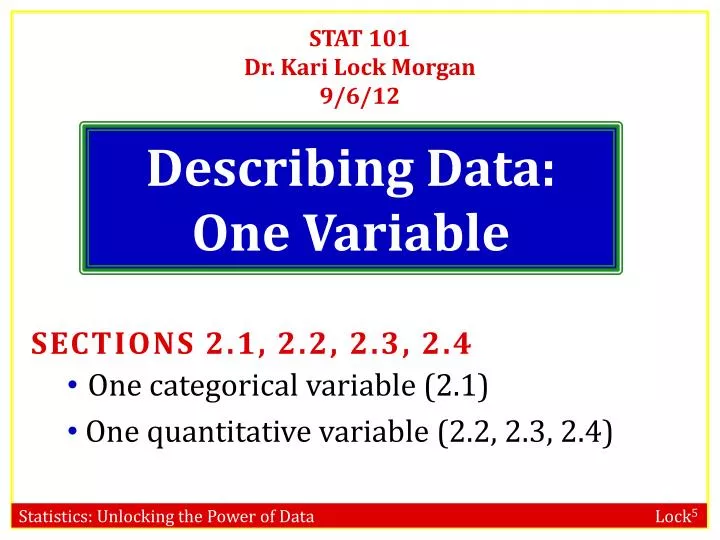
STAT 101 Dr. Kari Lock Morgan 9/6/12. Describing Data: One Variable. SECTIONS 2.1, 2.2, 2.3, 2.4 One categorical variable (2.1) One quantitative variable (2.2, 2.3, 2.4). The Big Picture. Sample. Population. Sampling. Statistical Inference. Descriptive Statistics.

E N D
STAT 101 Dr. Kari Lock Morgan 9/6/12 Describing Data: One Variable • SECTIONS 2.1, 2.2, 2.3, 2.4 • One categorical variable (2.1) • One quantitative variable (2.2, 2.3, 2.4)
The Big Picture Sample Population Sampling Statistical Inference Descriptive Statistics
Descriptive Statistics • In order to make sense of data, we need ways to summarize and visualize it • Summarizing and visualizing variables and relationships between two variables is often known as descriptive statistics (also known as exploratory data analysis) • Type of summary statistics and visualization methods depend on the type of variable(s) being analyzed (categorical or quantitative)
One Categorical Variable • A random sample of US adults in 2012 were surveyed regarding the type of cell phone owned • Android? iPhone? Blackberry? Non-smartphone? No cell phone?
Frequency Table • A frequency tableshows the number of cases that fall in each category: R: table(x)
Proportion The proportionin a category is found by • Proportion for a sample: (“p-hat”) • Proportion for a population: p
Proportion • What proportion of adults sampled do not own a cell phone? or 13% Proportions and percentages can be used interchangeably
Relative Frequency Table • A relative frequency tableshows the proportion of cases that fall in each category • All the numbers in a relative frequency table sum to 1 R: table(x)/length(x)
Bar Chart/Plot/Graph • In a barplot, the height of the bar corresponds to the number of cases falling in each category R: barchart(x)
Pie Chart • In a pie chart, the relative area of each slice of the pie corresponds to the proportion in each category R: pie(table(x))
StatKey www.lock5stat.com/statkey
Summary: One Categorical Variable • Summary Statistics • Proportion • Frequency table • Relative frequency table • Visualization • Bar chart • Pie chart
One Quantitative Variable World gross for all 2011 Hollywood movies HollywoodMovies2011 • More graphics on profits for Hollywood movies
Dotplot • In a dotplot, each case is represented by a dot and dots are stacked. • Easy way to see each case
Histogram • The height of the each bar corresponds to the number of cases within that range of the variable R: hist(x)
Histogram vs Bar Chart This is a • Histogram • Bar chart • Other • I have no idea
Histogram vs Bar Chart This is a • Histogram • Bar chart • Other • I have no idea
Histogram vs Bar Chart • A bar chart is for categorical data, and the x-axis has no numeric scale • A histogram is for quantitative data, and the x-axis is numeric • For a categorical variable, the number of bars equals the number of categories, and the number in each category is fixed • For a quantitative variable, the number of bars in a histogram is up to you (or your software), and the appearance can differ with different number of bars
Shape Long right tail Symmetric Right-Skewed Left-Skewed
Notation • The sample size, the number of cases in the sample, is denoted by n • We often let x or y stand for any variable, and x1 , x2 , …, xnrepresent the n values of the variable x • x1= 97.009, x2= 201.897, x3 = 216.196, …
Mean The mean or average of the data values is • Sample mean: • Population mean: (“mu”) R: mean(x)
Median The median, m, is the middle value when the data are ordered. If there are an even number of values, the median is the average of the two middle values. • The median splits the data in half. R: median(x)
Measures of Center m = 76.66 =150.74 Mean is “pulled” in the direction of skewness World Gross (in millions)
Skewness and Center A distribution is left-skewed. Which measure of center would you expect to be higher? • Mean • Median The mean will be pulled down towards the skewness (towards the long tail).
Outlier An outlier is an observed value that is notably distinct from the other values in a dataset.
Outliers Harry Potter Transformers Pirates of the Caribbean World Gross (in millions)
Resistance A statistic is resistant if it is relatively unaffected by extreme values. • The median is resistant while the mean is not.
Outliers • When using statistics that are not resistant to outliers, stop and think about whether the outlier is a mistake • If not, you have to decide whether the outlier is part of your population of interest or not • Usually, for outliers that are not a mistake, it’s best to run the analysis twice, once with the outlier(s) and once without, to see how much the outlier(s) are affecting the results
Standard Deviation The standard deviationfor a quantitative variable measures the spread of the data • Sample standard deviation: s • Population standard deviation: (“sigma”) R: sd(x)
Standard Deviation • The standard deviation gives a rough estimate of the typical distance of a data values from the mean • The larger the standard deviation, the more variability there is in the data and the more spread out the data are
Standard Deviation Both of these distributions are bell-shaped
95% Rule If a distribution of data is approximately symmetric and bell-shaped, about 95% of the data should fall within two standard deviations of the mean. • For a population, 95% of the data will be between µ – 2 and µ + 2 • StatKey
The 95% Rule The standard deviation for hours of sleep per night is closest to • ½ • 1 • 2 • 4 • I have no idea
z-score The z-score for a data value, x, is • For a population, is replaced with µ and s is replaced with • Values farther from 0 are more extreme
z-score • A z-score puts values on a common scale • A z-score is the number of standard deviations a value falls from the mean • 95% of all z-scores fall between what two values? • z-scores beyond -2 or 2 can be considered extreme -2 and 2
z-score Which is better, an ACT score of 28 or a combined SAT score of 2100? • ACT: = 21, = 5 • SAT: = 1500, = 325 • Assume ACT and SAT scores have approximately bell-shaped distributions • ACT score of 28 • SAT score of 2100 • I don’t know
Other Measures of Location • Maximum = largest data value • Minimum = smallest data value • Quartiles: • Q1 = median of the values below m. • Q3 = median of the values above m.
Min Q1 m Q3 Max 25% 25% 25% 25% Five Number Summary • Five Number Summary: R: summary(x)
Five Number Summary The distribution of number of hours spent studying each week is • Symmetric • Right-skewed • Left-skewed • Impossible to tell > summary(study_hours) Min. 1st Qu. Median 3rd Qu. Max. 2.00 10.00 15.00 20.00 69.00
Percentile The Pthpercentileis the value which is greater than P% of the data • We already used z-scores to determine whether an SAT score of 2100 or an ACT score of 28 is better • We could also have used percentiles: • ACT score of 28: 91st percentile • SAT score of 2100: 97th percentile
Min Q1 m Q3 Max 25% 25% 25% 25% Five Number Summary • Five Number Summary: 50th percentile 75th percentile 100th percentile 0th percentile 25th percentile
Measures of Spread • Range = Max – Min • Interquartile Range (IQR)= Q3 – Q1 • Is the range resistant to outliers? • Yes • No • Is the IQR resistant to outliers? • Yes • No The range depends entirely on the most extreme values. The IQR is based off the middle 50% of the data, which will not contain outliers.
Comparing Statistics • Measures of Center: • Mean (not resistant) • Median (resistant) • Measures of Spread: • Standard deviation (not resistant) • IQR (resistant) • Range (not resistant) • Most often, we use the mean and the standard deviation, because they are calculated based on all the data values, so use all the available information
Outliers • Outliers can be informally identified by looking at a plot, but one rule of thumb for identifying outliers is data values more than 1.5 IQRs beyond the quartiles • A data value is an outlier if it is Smaller than Q1 – 1.5(IQR) or Larger than Q3 + 1.5(IQR)
Boxplot Outliers • Lines (“whiskers”) extend from each quartile to the most extreme value that is not an outlier Q3 Median Q1 R: boxplot(x)
Boxplot Which boxplot goes with the histogram of waiting times for the bus? (a) (b) (c) The data do not show any low outliers.
StatKey www.lock5stat.com/statkey
Summary: One Quantitative Variable • Summary Statistics • Center: mean, median • Spread: standard deviation, range, IQR • Percentiles • 5 number summary • Visualization • Dotplot • Histogram • Boxplot • Other concepts • Shape: symmetric, skewed, bell-shaped • Outliers, resistance • z-scores